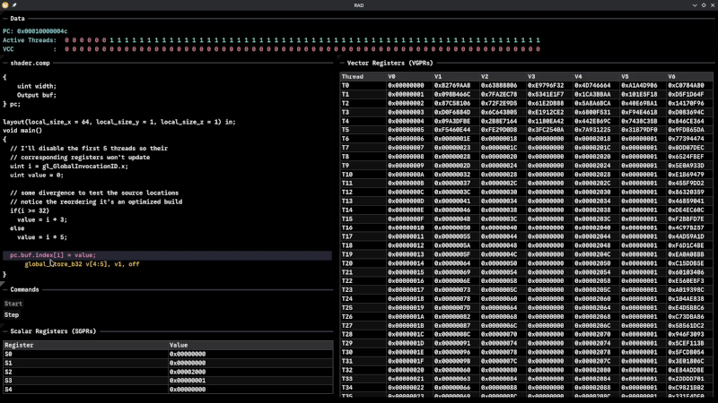
Although Robert F. Kennedy gets the credit for popularizing it, George Bernard Shaw said: “Some men see things as they are and say, ‘Why?’ I dream of things that never were and say, ‘Why not?'” Well, [Hadz] didn’t wonder why there weren’t many GPU debuggers. Instead, [Hadz] decided to create one.
It wasn’t the first; he found some blog posts by [Marcell Kiss] that helped, and that led to a series of experiments you’ll enjoy reading about. Plus, don’t miss the video below that shows off a live demo.
It seems that if you don’t have an AMD GPU, this may not be directly useful. But it is still a fascinating peek under the covers of a modern graphics card. Ever wonder how to interact with a video card without using something like Vulkan? This post will tell you how.
Writing a debugger is usually a tricky business anyway. Working with the strange GPU architecture makes it even stranger. Traps let you gain control, but implementing features like breakpoints and single-stepping isn’t simple.
We’ve used things like CUDA and OpenCL, but we haven’t been this far down in the weeds. At least, not yet. CUDA, of course, is specific to NVIDIA cards, isn’t it?
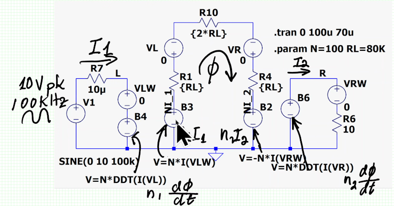
[Sam Ben-Yaakov] has another lecture online that dives deep into the physics of electronic processes. This time, the subject is magnetic transformers. You probably know that the ratio of current in the primary and secondary is the same (ideally) as the ratio of the turns in each winding. But do you know why? You will after watching the video.
Actually, you will after watching the first two minutes of the video. If you make it to the 44-minute mark, you’ll learn more about Faraday’s law, conservation of energy, and Lenz’s law.
One of our favorite things about the Internet is that you can find great lectures like these online, both from university programs and from individuals like [Dr. Ben-Yaakov]. There was a time when you would have had to enroll in a college to get the kind of education you can just browse through now.
Too much math and technical detail for you? We get it. You don’t need to understand all of this to use a transformer. But if you want to understand the math and the physics behind the things we do, nothing is stopping you. Even if you need to brush up on math, there are plenty of similar lectures to learn about that online, too.
Want a university class that is more practical? We hear you. Prefer simulation to math or solder? We hear you, too.
We noted that Excel turned 40 this year. That makes it seem old, and today, if you say “spreadsheet,” there’s a good chance you are talking about an Excel spreadsheet, and if not, at least a program that can read and produce Excel-compatible sheets. But we remember a time when there was no Excel. But there were still spreadsheets. How far back do they go?
Definitions
Like many things, exactly what constitutes a spreadsheet can be a little fuzzy. However, in general, a spreadsheet looks like a grid and allows you to type numbers, text, and formulas into the cells. Formulas can refer to other cells in the grid. Nearly all spreadsheets are smart enough to sort formulas based on which ones depend on others.
For example, if you have cell A1 as Voltage, and B1 as Resistance, you might have two formulas: In A2 you write “=A1/B1” which gives current. In B2 you might have “=A1*A2” which gives power. A smart spreadsheet will realize that you can’t compute B2 before you compute A2. Not all spreadsheets have been that smart.
There are other nuances that many, but not all, spreadsheets share. Many let you name cells, so you can simply type =VOLTS*CURRENT. Nearly all will let you specify absolute or relative references, too. With a relative reference, you might compute cell D1=A1*B1. If you copy this to row two, it will wind up D2=A2*B2. However, if you mark some of the cells absolute, that won’t be true. For example, copying D1=A1*$B$1 to row two will result in D2=A2*$B$1.
Not all spreadsheets mark rows and columns the same way, but the letter/number format is nearly universal in modern programs. Many programs still support RC references, too, where R4C2 is row four, column two. In that nomenclature, R[-1]C[2] is a relative reference (one row back, two rows to the right). But the real idea is that you can refer to a cell, not exactly how you refer to it.
So, How Old Are They?
LANPAR was probably the first spreadsheet program, and it was available for the GE400. The name “LANPAR” was LANguage for Programming Arrays at Random, but was also a fusion of the authors’ names. Want to guess the year? 1969. Two Harvard graduates developed it to solve a problem for the Canadian phone company’s budget worksheets, which took six to twenty-four months to change in Fortran. The video below shows a bit of the history behind LANPAR.
LANPAR might not be totally recognizable as a modern spreadsheet, but it did have cell references and proper order of calculations. In fact, they had a patent on the idea, although the patent was originally rejected, won on appeal, and later deemed unenforceable by the courts.
There were earlier, noninteractive, spreadsheet-like programs, too. Richard Mattessich wrote a 1961 paper describing FORTRAN IV methods to work with columns or rows of numbers. That generated a language called BCL (Business Computer Language). Others over the years included Autoplan, Autotab, and several other batch-oriented replacements for paper-based calculations.
Spreadsheets Get Personal
Back in the late 1970s, people like us speculated that “one day, every home would have a computer!” We just didn’t know what people would do with them outside of the business context where the computer lived at the time. We imagined people scaling up and down cooking recipes, for example. Exactly how do you make soup for nine people when the recipe is written for four? We also thought they might balance their checkbook or do math homework.
The truth is, two programs drove massive sales of small computers: WordStar, a word-processing program, and VisiCalc. Originally for the Apple ][, Visicalc by Dan Bricklin and Bob Frankston put desktop computers on the map, especially for businesses. VisiCalc was also available on CP/M, Atari computers, and the Commodore PET.
You’d recognize VisiCalc as a spreadsheet, but it did have some limitations. For one, it did not follow the natural order of operations. Instead, it would start at the top, work down a column, and then go to the next column. It would then repeat the process until no further change occurred.
However, it did automatically recalculate when you made changes, had relative and absolute references, and was generally interactive. You could copy ranges, and the program doesn’t look too different from a modern spreadsheet.
Sincere Flattery
Of course, once you have VisiCalc, you are going to invite imitators. SuperCalc paired with WordStar became very popular among the CP/M crowd. Then came the first of the big shots: Lotus 1-2-3. In 1982, this was a must-have application for the new IBM PC.
There were other contenders, each with its own claims to fame. Innovative Software’s SMART suite, for example, was among the first spreadsheets that let you have formulas that crossed “tabs.” It could also recalculate repeatedly until meeting some criteria, for example, recalculate until cell X20 is less than zero.
Probably the first spreadsheet that could handle multiple sheets to form a “3D spreadsheet” was BoeingCalc. Yes, Boeing like the aircraft. They had a product that ran on PCs or IBM 4300 mainframes. It used virtual memory and could accommodate truly gigantic sheets for its day. It was also pricey, didn’t provide graphics out of the box, and was slow. The Infoworld’s standard spreadsheet took 42.9 seconds to recalculate, versus 7.9 for the leading competitor at the time. Quatro Pro from Borland was also capable of large spreadsheets and provided tabs. It was used more widely, too.
Then Came Microsoft
Of course, the real measure of success in software is when the lawsuits start. In 1987, Lotus sued two spreadsheet companies that made very similar products (TWIN and VP Planner). Not to be outdone, VisiCalc’s company (Software Arts) sued Lotus. Lotus won, but it was a pyrrhic victory as Microsoft took all the money off the table, anyway.
Before the lawsuits, in 1985, Microsoft rolled out Excel for the Mac. By 1987, they also ported it to the fledgling Windows operating system. Of course, Windows exploded — make your own joke — and by the time Lotus 1-2-3 could roll out Windows versions, they were too late. By 2013, Lotus 1-2-3, seemingly unstoppable a few years earlier, fell to the wayside.
There are dozens of other spreadsheet products that have come and gone, and a few that still survive, such as OpenOffice and its forks. Quattro Pro remains available (as part of WordPerfect). You can find plenty of spreadsheet action in any of the software or web-based “office suites.”
Today and the Future
While Excel is 40, it isn’t even close to the oldest of the spreadsheets. But it certainly has kept the throne as the most common spreadsheet program for a number of years.
Many of the “power uses” of spreadsheets, at least in engineering and science, have been replaced by things like Jupyter Notebooks that let you freely mix calculations with text and graphics along with code in languages like Python, for example.
If you want something more traditional that will still let you hack some code, try Grist. We have to confess that we’ve abused spreadsheets for DSP and computer simulation. What’s the worst thing you’ve done with a spreadsheet?
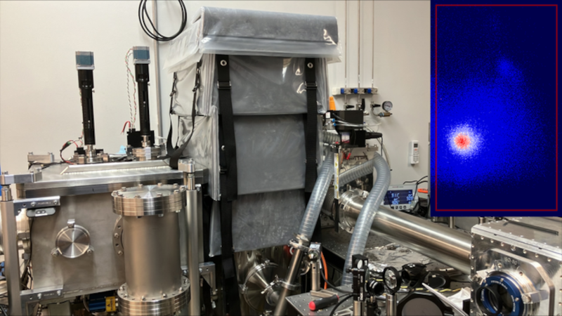
If you have ever thought, “I wish I could have a mass spectrometer at home,” then we aren’t very surprised you are reading Hackaday. [Thomas Scherrer] somehow acquired a broken Brucker Microflex LT Mass Spectrometer, and while it was clearly not working, it promised to be a fun teardown, as you can see in the first part of the video below.
Inside are lasers and definitely some high voltages floating around. This appears to be an industrial unit, but it has a great design for service. Many of the panels are removable without tools.
The construction is interesting in that it looks like a rack, but instead of rack mounting, everything is mounted on shelves. The tall unit isn’t just for effect. The device has a tall column where it measures the sample under test. The measurement is a time of flight so the column has to be fairly long to get results.
The large fiber laser inside produces a 100 kW pulse, which sounds amazing, but it only lasts for 2.5 ns. There’s also a “smaller” 10W laser in the unit.
There are also vacuum pumps and other wizardry inside. Check out the video and get a glimpse into something you aren’t likely to have a chance to tear into yourself. There are many ways to do mass spectrometry, and some of them are things you could build yourself. We’ve seen it done more than once.
Admit it or not, you probably have a teddy bear somewhere in your past that you were — or maybe are — fond of. Not to disparage your bear, but we think Bradfield might have had a bigger adventure than yours has. Bradfield was launched in November on a high-altitude balloon by Year 7 and 8 students at Walhampton School in the UK in connection with Southampton University. Dressed in a school uniform, he was supposed to ride to near space, but ran into some turbulence. The BBC reported that poor Bradfield couldn’t hold on any longer and fell from around 17 miles up. The poor bear looked fairly calm for being so high up.
A camera recorded the unfortunate stuffed animal’s plight. Apparently, a companion plushie, Bill the Badger (the Badger being the Southampton mascot), successfully completed the journey, returning to Earth with a parachute.
There have been some news reports that Bradfield may have been recovered, but we haven’t seen anything definitive yet. Of course, there are plenty of things you can launch on a balloon, but what a great idea to let kids send a mascot aloft with your serious science payloads and radio gear. Because we know you are launching a balloon for a serious purpose, right? Sure, we won’t tell you just want the cool pictures.
No offense to Bradfield, but sending humans aloft on balloons requires a little more care. We aren’t as well-equipped to drop 17 miles. The Hackaday Supercon has even been the site of an uncrewed (and unbeared) balloon launch. Meanwhile, if you are around Reading and spot Bradfield, be sure to give him a cookie and call the Walhampton school.
Hackaday Editors Elliot Williams and Al Williams met up to cover the best of Hackaday this week, and they want you to listen in. There were a hodgepodge of hacks this week, ranging from home automation with RF, volumetric displays in glass, and some crazy clocks, too.
Ever see a typewriter that uses an ink pen? Elliot and Al hadn’t either. Want time on a supercomputer? It isn’t free, but it is pretty cheap these days. Finally, the guys discussed how to focus on a project like Dan Maloney, who finally got a 3D printer, and talked about Maya Posch’s take on LLM intelligence.
Check out the links below if you want to follow along, and as always, tell us what you think about this episode in the comments!
If you get a chance to visit a computer history museum and see some of the very old computers, you’ll think they took up a full room. But if you ask, you’ll often find that the power supply was in another room and the cooling system was in yet another. So when you get a computer that fit on, say, a large desk and maybe have a few tape drives all together in a normal-sized office, people thought of it as “small.” We’re seeing a similar evolution in particle accelerators, which, a new startup company says, can be room-sized according to a post by [Charles Q. Choi] over at IEEE Spectrum.
Usually, when you think of a particle accelerator, you think of a giant housing like the 3.2-kilometer-long SLAC accelerator. That’s because these machines use magnets to accelerate the particles, and just like a car needs a certain distance to get to a particular speed, you have to have room for the particle to accelerate to the desired velocity.
A relatively new technique, though, doesn’t use magnets. Instead, very powerful (but very short) laser pulses create plasma from gas. The plasma oscillates in the wake of the laser, accelerating electrons to relativistic speeds. These so-called wakefield accelerators can, in theory, produce very high-energy electrons and don’t need much space to do it.
The startup company, TAU Systems, is about to roll out a commercial system that can generate 60 to 100 MeV at 100 Hz. They also intend to increase the output over time. For reference, SLAC generates 50,000 MeV. But, then again, it takes two miles of raceway to do it.
The initial market is likely to be radiation testing for space electronics. Higher energies will open the door to next-generation X-ray lithography for IC production, and more. There are likely applications for accelerated electrons that we don’t see today because it isn’t feasible to generate them without a massive facility.
On the other hand, don’t get your checkbook out yet. The units will cost about $10 million at the bottom end. Still a bargain compared to the alternatives.
For as long as there have been supercomputers, people like us have seen the announcements and said, “Boy! I’d love to get some time on that computer.” But now that most of us have computers and phones that greatly outpace a Cray 2, what are we doing with them? Of course, a supercomputer today is still bigger than your PC by a long shot, and if you actually have a use case for one, [Stephen Wolfram] shows you how you can easily scale up your processing by borrowing resources from the Wolfram Compute Services. It isn’t free, but you pay with Wolfram service credits, which are not terribly expensive, especially compared to buying a supercomputer.
[Stephen] says he has about 200 cores of local processing at his house, and he still sometimes has programs that run overnight. If your program already uses a Wolfram language and uses parallelism — something easy to do with that toolbox — you can simply submit a remote batch job.
What constitutes a supercomputer? You get to pick. You can just offload your local machine using a single-core 8GB virtual machine — still a supercomputer by 1980s standards. Or you get machines with up to 1.5TB of RAM and 192 cores. Not enough for your mad science? No worries, you can map a computation across more than one machine, too.
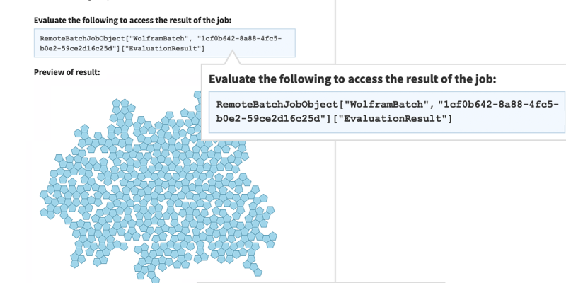
As an example, [Stephen] shows a simple program that tiles pentagons:
When the number of pentagons gets large, a single line of code sends it off to the cloud:
RemoteBatchSubmit[PentagonTiling[500]]
The basic machine class did the work in six minutes and 30 seconds for a cost of 5.39 credits. He also shows a meatier problem running on a 192-core 384GB machine. That job took less than two hours and cost a little under 11,000 credits (credit cost from just over $4/1000 to $6/1000, depending on how many you buy, so this job cost about $55 to run). If two hours is too much, you can map the same job across many small machines, get the answer in a few minutes, and spend fewer credits in the process.
Supercomputers today are both very different from old supercomputers and yet still somewhat the same. If you really want that time on the Cray you always wanted, you might think about simulation.
NVMe solid state disk drives have become inexpensive unless you want the very largest sizes. But how do you get the most out of one? There are two basic strategies: you can use the drive as a fast drive for things you use a lot, or you can use it to cache a slower drive.
Each method has advantages and disadvantages. If you have an existing system, moving high-traffic directories over to SSD requires a bind mount or, at least, a symbolic link. If your main filesystem uses RAID, for example, then those files are no longer protected.
Caching sounds good, in theory, but there are at least two issues. You generally have to choose whether your cache “writes through”, which means that writes will be slow because you have to write to the cache and the underlying disk each time, or whether you will “write back”, allowing the cache to flush to disk occasionally. The problem is, if the system crashes or the cache fails between writes, you will lose data.
Compromise
For some time, I’ve adopted a hybrid approach. I have an LVM cache for most of my SSD that hides the terrible performance of my root drive’s RAID array. However, I have some selected high-traffic, low-importance files in specific SSD directories that I either bind-mount or symlink into the main directory tree. In addition, I have as much as I can in tmpfs, a RAM drive, so things like /tmp don’t hit the disks at all.
There are plenty of ways to get SSD caching on Linux, and I won’t explain any particular one. I’ve used several, but I’ve wound up on the LVM caching because it requires the least odd stuff and seems to work well enough.
This arrangement worked just fine and gives you the best of both worlds. Things like /var/log and /var/spool are super fast and don’t bog down the main disk. Yet the main disk is secure and much faster thanks to the cache setup. That’s been going on for a number of years until recently.
The Upgrade Issue
I recently decided to give up using KDE Neon on my main desktop computer and switch to OpenSUSE Tumbleweed, which is a story in itself. The hybrid caching scheme seemed to work, but in reality, it was subtly broken. The reason? SELinux.
Tumbleweed uses SELinux as a second level of access protection. On vanilla Linux, you have a user and a group. Files have permissions for a specific user, a specific group, and everyone else. Permission, in general, means if a given user or group member can read, write, or execute the file.
SELinux adds much more granularity to protection. You can create rules that, for example, allow certain processes to write to a directory but not read from it. This post, though, isn’t about SELinux fundamentals. If you want a detailed deep dive from Red Hat, check out the video below.
The Problem
The problem is that when you put files in SSD and then overlay them, they live in two different places. If you tell SELinux to “relabel” files — that is, put them back to their system-defined permissions, there is a chance it will see something like /SSD/var/log/syslog and not realize that this is really the same file as /var/log. Once you get the wrong label on a system file like that, bad, unpredictable things happen.
There is a way to set up an “equivalence rule” in SELinux, but there’s a catch. At first, I had the SSD mounted at /usr/local/FAST. So, for example, I would have /usr/local/FAST/var/log. When you try to equate /usr/local/FAST/var to /usr/var, you run into a problem. There is already a rule that /usr and /usr/local are the same. So you have difficulties getting it to understand that throws a wrench in the works.
There are probably several ways to solve this, but I took the easy way out: I remounted to /FAST. Then it was easy enough to create rules for /var/log to /FAST/var/log, and so on. To create an equivalence, you enter:
semanage fcontext -a -e /var/log /FAST/var/log
The Final Answer
So what did I wind up with? Here’s my current /etc/fstab:
Note that some of these don’t appear in /etc/fstab because they are symlinks.
A good rule of thumb is that if you ask SELinux to relabel the tree in the “real” location, it shouldn’t change anything (once everything is set up). If you see many changes, you probably have a problem:
restorecon -Rv /FAST/var/log
Worth It?
Was it worth it? I can certainly feel the difference in the system when I don’t have this setup, especially without the cache. The noisy drives quiet down nicely when most of the normal working set is wholly enclosed in the cache.
This setup has worked well for many years, and the only really big issue was the introduction of SELinux. Of course, for my purposes, I could probably just disable SELinux. But it does make sense to keep it on if you can manage it.
If you have recently switched on SELinux, it is useful to keep an eye on:
ausearch -m AVC -ts recent
That shows you if SELinux denied any access recently. Another useful command:
systemctl status setroubleshootd.service
Another good systemd “stupid trick.” Often, any mysterious issues will show up in one of those two places. If you are on a single-user desktop, it isn’t a bad idea to retry any strange anomalies with SELinux turned off as a test: setenforce 0. If the problem goes away, it is a sure bet that something is wrong with the SELinux system.
Of course, every situation is different. If you don’t need RAID or a huge amount of storage, maybe just use an SSD as your root system and be done with it. That would certainly be easier. But, in typical Linux fashion, you can make of it whatever you want. We like that.
Today, it is hard to imagine a world without recorded audio, and for the most part that started with Edison’s invention of the phonograph. However, for most of its history, the phonograph was a one-way medium. Although early phonographs could record with a separate needle cutting into foil or wax, most record players play only records made somewhere else. The problem is, this cuts down on what you can do with them. When offices were full of typists and secretaries, there was the constant problem of telling the typist what to type. Whole industries developed around that problem, including the Dictaphone company.
The issue is that most people can talk faster than others can write or type. As a result, taking dictation is frustrating as you have to stop, slow down, repeat yourself, or clarify dubious words. Shorthand was one way to equip a secretary to write as fast as the boss can talk. Steno machines were another way. But the dream was always a way to just speak naturally, at your convenience, and somehow have it show up on a typewritten page. That’s where the Dictaphone company started.
History of the Dictaphone
Unsurprisingly, Dictaphone’s founder was the famous Alexander Graham Bell. Although Edison invented the phonograph, Bell made many early improvements to the machine, including the use of wax instead of foil as a recording medium. He actually started the Volta Graphophone Company, which merged with the American Graphophone Company that would eventually become Columbia Records.
In 1907, the Columbia Phonograph Company trademarked the term Dictaphone. While drum-based machines were out of style in other realms, having been replaced by platters, the company wanted to sell drum-based machines that let executives record audio that would be played back by typists. By 1923, the company spun off on its own.
Edison, of course, also created dictation machines. There were many other companies that made some kind of dictation machine, but Dictaphone became the standard term for any such device, sort of like Xerox became a familiar term for any copier.
Dictaphones were an everyday item in early twentieth-century offices for dictation, phone recording, and other audio applications. Not to mention a few other novel uses. In 1932, a vigilante organization used a Dictaphone to bug a lawyer’s office suspected of being part of a kidnapping.
Some machines could record and playback. Others, usually reserved for typists, were playback-only. In addition, some machines could “shave” wax cylinders to erase a cylinder for future use. Of course, eventually you’d shave it down to the core, and then it was done.
The Computer History Archives has some period commercials and films from Dictaphone, and you can see them in the videos below.
As mentioned, Dictaphone wasn’t the only game in town. Edison was an obvious early competitor. We were amused that the Edison devices had a switch that allowed them to operate on AC or DC current.
Later, other companies like IBM would join in. Some, like the Gray Audograph and the SoundScriber used record-like disks instead of belts or drums. Of course, eventually, magnetic tape cassettes were feasible, too, and many people made recorders that could be used for dictation and many other recording duties.
The Dictabelt
For the first half of the twentieth century, Dictaphones used wax cylinders. However, in 1947, they began making machines that pressed a groove into a Lexan belt — a “Dictabelt,” at first called a “Memobelt.” These were semi-permanent and, since you couldn’t easily melt over some of the wax, difficult to tamper with, which helped make them admissible in court. Apparently, you could play a Dictabelt back about 20 times before it would be too beat up to play.
These belts found many uses. For one, Dictaphone was a major provider to police departments and other similar services, recording radio traffic and telephone calls. In the late 1970s, the House Select Committee on Assassinations used Dictaphone belts from the Dallas police department recording in 1963 to do audio analysis on the Kennedy assassination. Many Dictaphones found homes in courtrooms, too.
As you can see in the commercials in the video, Dictabelts would fit in an envelope: they are about 3.5 in x 12 in or 89 mm x 300 mm. The “portable” machine promised to let you dictate from anywhere, keep meeting minutes, and more. A single belt held 15 minutes of audio, and the color gives you an idea of when the belt was made.
Magnetic Personality
Of course, Dictaphone wasn’t the only game in town for machines like this. IBM released one that used a magnetic belt called a “Magnabelt’ that you could edit. Dictaphone followed suit. These, of course, were erasable.
Even as late as 1977, you could find Dictaphones in “word processing operations” like the one in the video with the catchy tune, below. Of course, computers butted into both word processing and dictation with products like Via Voice or DragonDictate. Oddly, DragonDictate is from Nuance, which bought what was left of Dictaphone.
Insides
Since this is Hackaday, of course, you want to see the insides of some of these machines. A video from [databits] gives us a peek below.
Offices have certainly changed. Most people do their own typing now. Your phone can record many hours of crystal-clear audio. Computers can even take your dictation now, if you insist.
Should you ever find a Dictabelt and want to digitize it for posterity, you might find the video below from [archeophone] useful. They make a modern playback unit for old cylinders and belts.
We’d love to see a homebrew Dictabelt recorder player using more modern tech. If you make one, be sure to let us know. People recorded on the darndest things. Tape caught on primarily because of World War II Germany and Bing Crosby.
[Alexwlchan] noticed something funny. He knew that not putting a size for a video embedded in a web page would cause his page to jump around after the video loaded. So he put the right numbers in. But with some videos, the page would still refresh its layout. He learned that not all video sizes are equal and not all pixels are square.
For a variety of reasons, some videos have pixels that are rectangular, and it is up to your software to take this into account. For example, when he put one of the suspect videos into QuickTime Player, it showed the resolution was 1920×1080 (1350×1080). That’s the non-square pixel.
So just pulling the size out of a video isn’t always sufficient to get a real idea of how it looks. [Alex] shows his old Python code that returns the incorrect number and how he managed to make it right. The mediainfo library seems promising, but suffers from some rounding issues. Instead, he calls out to ffprobe, an external program that ships with ffmpeg. So even if you don’t use Python, you can do the same trick, or you could go read the ffprobe source code.
[Alex] admits that there are not many videos that have rectangular pixels, but they do show up.
Plotters aren’t as common as they once were. Today, many printers can get high enough resolution with dots that drawing things with a pen isn’t as necessary as it once was. But certainly you’ve at least seen or heard of machines that would draw graphics using a pen. Most of them were conceptually like a 3D printer with a pen instead of a hotend and no real Z-axis. But as [biosrhythm] reminds us, some plotters were suspiciously like typewriters fitted with pens.
Instead of type bars, type balls, or daisy wheels, machines like the Panasonic Penwriter used a pen to draw your text on the page, as you can see in the video below. Some models had direct computer control via a serial port, if you wanted to plot using software. At least one model included a white pen so you could cover up any mistakes.
If you didn’t have a computer, the machine had its own way to input data for graphs. How did that work? Read for yourself.
Panasonic wasn’t the only game in town, either. Silver Reed — a familiar name in old printers — had a similar model that could connect via a parallel port. Other familiar names are Smith Corona, Brother, Sharp, and Sears.
Since all the machines take the same pens, they probably have very similar insides. According to the post, Alps was the actual manufacturer of the internal plotting mechanism, at least.
The video doesn’t show it, but the machines would draw little letters just as well as graphics. Maybe better since you could change font sizes and shapes without switching a ball. They could even “type” vertically or at an angle, at least with external software.
Since plotters are, at heart, close to 3D printers, it is pretty easy to build one these days. If plotting from keystrokes is too mundane for you, try voice control.
[Engineezy] might have been watching a 3D printer move when inspiration struck: Why not build a robot arm to clean up his workbench? Why not, indeed? Well, all you need is a 17-foot-long X-axis and a gripper mechanism that can pick up any strange thing that happens to be on the bench.
Like any good project, he did it step by step. Mounting a 17-foot linear rail on an accurately machined backplate required professional CNC assistance. He was shooting for a 1mm accuracy, but decided to settle for 10mm.
With the long axis done, the rest seemed anticlimactic, at least for moving it around. The system can actually support his bodyweight while moving. The next step was to control the arm manually and use a gripper to open a parts bin.
The arm works, but is somewhat slow and needs some automation. A great start to a project that might not be practical, but is still a fun build and might inspire you to do something equally large.
We have large workbenches, but we tend to use tiny ones more often in our office. We also enjoy ones that are portable.
Color 3D printing has gone mainstream, and we expect more than one hacker will be unpacking one over the holidays. If you have, say, a color inkjet printer, the process is simple: print. Sure, maybe make sure you tick the “color” box, but that’s about it. However, 3D printers are a bit more complicated.
There are two basic phases to printing color 3D prints. First, you have to find or make a model that has different colors. Even if you don’t make your own models (although you should), you can still color prints in your slicer.
The second task is to set the printer up to deal with those multiple colors. There are several different ways to do this, and each one has its pros and cons. Of course, some of this depends on your slicer, and some depends on your printer. For the purposes of this post, I’ll assume you are using a Slic3r fork like Prusa or OrcaSlicer. Most of the lower-priced printers these days work in roughly the same way.
Current State of Color
In theory, there are plenty of ways to 3D print in color. You can mix hot plastic in the nozzle or use multiple nozzles, each loaded with a different color. But most entry-level color printers use a variation of the same technique. Essentially, they are just like single-nozzle FDM printers, but they have three extra pieces. First, there is a sensor that can tell if filament is in the hot end or not. There’s also a blade above the hot end but below the extruder that can cut the filament off cleanly on command. This usually involves having the hot end ram some actuator that pushes the spring-loaded knife through the filament.
The third piece is some unit to manage moving a bunch of filaments in and out of the hot end. Everyone calls this something else. Bambu calls it an AMS while Flashforge calls it an IFS. Prusa has an MMU. Whatever you call it, it just moves cold filament around: either pushing it into the extruder or pulling it out.
Every filament change starts with cutting the filament below the extruder. That leaves the stringy melted part down in the nozzle. Then the extruder can pull the rest up until the management unit can take over and pull it totally out of the hot end/extruder assembly. That’s why there’s a sensor. It pulls until it sees that the extruder is empty or it times out and throws an error.
Then it is simple enough to move another filament back into the extruder. Of course, the first thing it has to do is push the leftover filament out of the nozzle. Most printers move to a bin and extrude until they are sure the color has changed. However, there are other options.
Even if you push out all the old filament, you may want to print a little waste piece of the new filament before you start printing, and this is called a purge block. Slicers can also push purge material into places like your infill, for example. Some can even print objects with the purge, presumably an object that doesn’t have to look very nice. Depending on your slicer, printer, and workflow, you can opt to print without a purge block, which can work well when you have a part where each layer is a solid color. Some printers will let you skip the discharge step, too, which is often called “poop.”
One caveat, of course, is that all this switching logic takes time and generates waste. A good rule of thumb is to try to print many objects at one time if you are going to switch filament, because the changes are what take time and generate waste. Printing dozens of objects will generate essentially the same amount of waste as printing one. Of course, printing a dozen objects will take longer than a single one, but the biggest part of the time is filament changes, which doesn’t change no matter how many or few you print.
Get Ready to Print
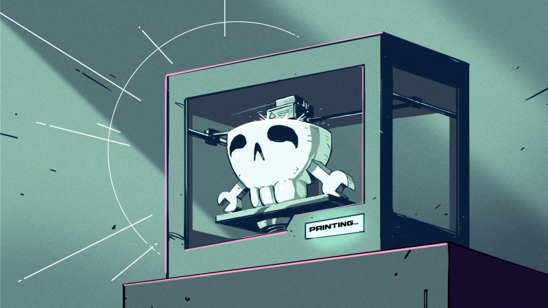
Painting in Orca Slicer
We’ve talked before about creating your own color objects. We’ve even seen how to do it in TinkerCad. Of course, you can also load designs that already have color in them. However, there are several different ways to put color into an otherwise monochrome print.
First, you can take a regular print and use your slicer’s paint function to paint areas with different colors. That works, but it is often tedious, and for complex shapes, it is error-prone. Another downside is that you can’t really control the depth easily, so you get strange filament shifts inside the object if you do it that way.
In Orca, you can select an object in the Prepare screen and then use N, or the toolbar, to bring up the paint color dialog. From there, you can pick a brush shape, pen size, and color. Then it is easy to just paint where you like by left-dragging. You can remove paint by pressing Shift while clicking or dragging. Press the little question mark at the bottom left to see other options.
Once you make a color print, the slicer will automatically place a purge block for you unless you turn it off. Assuming you use it, it is a good idea to drag it on the build plate to be closer to the print, which can shave a few minutes of travel time.
From Many, One
Possibly the easiest way, other than not printing in color, of course, is to have each part of the model that needs to be one color as a separate STL file, as we talked about in the previous post. You tell the slicer which part goes with which filament, and you are done.
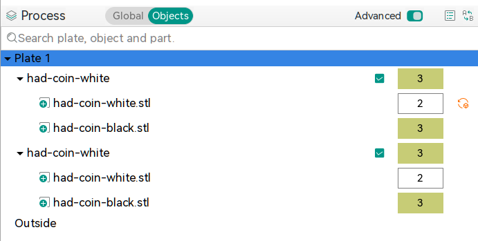
In Orca, the best way to do this is to import several STL models at one time. The software will ask you: “Load these files as a single object with multiple parts?” If you agree, you get one object made of individual pieces.
The resulting object won’t look much different until you go to “Process”, on the left-hand side of the screen, and switch from the default Global to Objects. From there, you’ll see the objects and their components. At first, each one will be set to the same color, but by clicking on the color box, you can assign different colors. In the screenshot, you’ll see two identical objects, each with two parts. Each part has a different color. The number is the extruder that holds that color.
Two filament changes are all it takes to make this nice-looking ornament
There is another way, though. You can avoid almost all of the waste generation and extra time if your model is designed so that each layer is a single color. People have done this for years, where you put a pause in your G-code and then switch filament manually. The idea is the same but the printer can switch for you. For example, the Christmas Tree ornament uses two filament changes to print white, then green, then white again. This works great for lettering and logos and other simple setups where you simply need some contrast.
In Orca, you’ll want to slice your model once and switch to the preview tab. Using the vertical slider on the right-hand side, adjust the view until it shows you where you want the filament change. Then right-click and select “Change Filament.” This is the same way you add a pause if you want to change filament manually, for example.
If you use this method, remember to turn off the purge block. You don’t really need it.
Summary
So now, when you unwrap that shiny new multimaterial printer, you have a plan. Get a color model or color one yourself. Then you can decide if you need color changes or full-blown, and waste-prone, color printing. Either way, have fun!
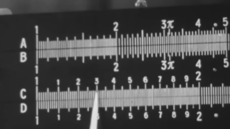
Learning something on YouTube seems kind of modern. But if you are watching a 1957 instructional film about slide rules, it also seems old-fashioned. But Encyclopædia Britannica has a complete 30-minute training film, which, what it lacks in glitz, it makes up for in mathematical rigor.
We appreciated that it started out talking about numbers and significant figures instead of jumping right into the slide rule. One thing about the slide rule is that you have to sort of understand roughly what the answer is. So, on a rule, 2×3, 20×30, 20×3, and 0.2×300 are all the same operation.
You don’t actually get to the slide rule part for about seven minutes, but it is a good idea to watch the introductory part. The lecturer, [Dr. Havery E. White] shows a fifty-cent plastic rule and some larger ones, including a classroom demonstration model. We were a bit surprised that the prestigious Britannica wouldn’t have a bit better production values, but it is clear. Perhaps we are just spoiled by modern productions.
We love our slide rules. Maybe we are ready for the collapse of civilization and the need for advanced math with no computers. If you prefer reading something more modern, try this post. Our favorites, though, are the cylindrical ones that work the same, but have more digits.
We love and hate OpenSCAD. As programmers, we like describing objects we want to 3D print or otherwise model. As programmers, we hate all the strange things about OpenSCAD that make it not like a normal programming language. Maybe µCAD (or Microcad) is the answer. This new entry in the field lets you build things programmatically and is written in Rust.
In fact, the only way to get it right now is to build it from source using cargo. Assuming you already have Rust, that’s not hard. Simply enter: cargo install microcad. If you don’t already have Rust, well, then that’s a problem. However, we did try to build it, and despite having the native library libmanifold available, Rust couldn’t find it. You might have better luck.
You can get a feel for the language by going through one of the tutorials, like the one for building a LEGO-like shape. Here’s a bit of code from that tutorial:
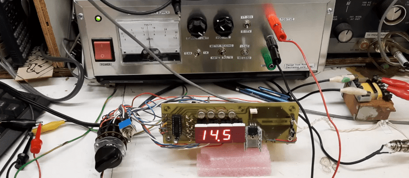
We can’t get enough of [Bettina Neumryn’s] videos. If you haven’t seen her, she takes old electronics magazines, finds interesting projects, and builds them. If you remember these old projects, it is nostalgic, and if you don’t remember them, you can learn a lot about basic electronics and construction techniques. This installment (see below) is an Elektor digital voltmeter and frequency counter from late 1981.
As was common in those days, you could find the PCB layouts in the magazine. In this case, there were two boards. The schematic shows that a counter and display driver chip — a 74C928 — does most of the heavy lifting for the display and the counter.
It is easy to understand how the frequency counter works. You clip the input with a pair of diodes, amplify it a bit, square it with a Schmitt trigger, and then, possibly, prescale it using a divider. The voltmeter is a little trickier: it uses a voltage divider, an op amp, and a 555 to convert the voltage to a frequency.
Of course, finding the parts for an old project can be a challenge. A well-stocked junk drawer doesn’t hurt. A PCB etching setup helps, too.
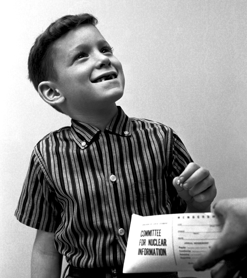
If you are a schoolkid of the right age, you can’t wait to lose a baby tooth. In many cultures, there is a ritual surrounding it, like the tooth fairy, a mouse who trades your tooth for a gift, or burying the tooth somewhere significant. But in 1958, a husband and wife team of physicians wanted children’s teeth for a far different purpose: quantifying the effects of nuclear weapons testing on the human body.
A young citizen scientist (State Historical Society of Missouri)
Louise and Eric Reiss, along with some other scientists, worked with Saint Louis University and the Washington School of Dental Medicine to collect and study children’s discarded teeth. They were looking for strontium-90, a nasty byproduct of above-ground nuclear testing. Strontium is similar enough to calcium that consuming it in water and dairy products will leave the material in your bones, including your teeth.
The study took place in the St. Louis area, and the results helped convince John F. Kennedy to sign the Partial Nuclear Test Ban Treaty.
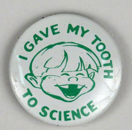
They hoped to gather 50,000 teeth in a year. By 1970, 12 years later, they had picked up over 320,000 donated teeth. While a few kids might have been driven by scientific altruism, it didn’t hurt that the program used colorful posters and promised each child a button to mark their participation.
Children’s teeth were particularly advantageous to use because they are growing and are known to readily absorb radioactive material, which can cause bone tumors.
Scale
A fair trade for an old tooth? (National Museum of American History)
You might wonder just how much nuclear material is floating around due to bombs. Obviously, there were two bombs set off during the war, as well as the test bombs required to get to that point. Between 1945 and 1980, there were five countries conducting atmospheric tests at thirteen sites. The US, accounting for about 65% of the tests, the USSR, the UK, France, and China detonated 504 nuclear devices equivalent to about 440 megatons of TNT.
Well over 500 bombs with incredible force have put a lot of radioactive material into the atmosphere. That doesn’t count, too, the underground tests that were not always completely contained. For example, there were two detonations in Mississippi where the radiation was contained until they drilled holes for instruments, leaving contaminated soil on the surface. Today, sites like this have “monuments” explaining that you shouldn’t dig in the area.
Of course, above-ground tests are worse, with fallout affecting “downwinders” or people who live downwind of the test site. There have been more than one case of people, unaware of the test, thinking the fallout particles were “hot snow” and playing in it. Test explosions have sent radioactive material into the stratosphere. This isn’t just a problem for people living near the test sites.
Results
By 1961, the team published results showing that strontium-90 levels in the teeth increased depending on when the child was born. Children born in 1963 had levels of strontium-90 fifty times higher than those born in 1950, when there was very little nuclear testing.
The results were part of the reason that President Kennedy agreed to an international partial test ban, as you can see in the Lincoln Presidential Foundation video below. You may find it amazing that people would plan trips to watch tests, and they were even televised.
In 2001, Washington University found 85,000 of the teeth stored away. This allowed the Radiation and Public Health Project to track 3,000 children who were, by now, adults, of course.
Sadly, 12 children who had died from cancer before age 50 had baby teeth with twice the levels of the teeth of people who were still alive at age 50. To be fair, the Nuclear Regulatory Commission has questioned these findings, saying the study is flawed and fails to account for other risk factors.
And teeth don’t just store strontium. In the 1970s, other researchers used baby teeth to track lead ingestion levels. Baby teeth have also played a role in the Flint Water scandal. In South Africa, the Tooth Fairy Project monitored heavy metal pollution in children’s teeth, too.
[Big Clive] picked up a tiny heater for less than £8 from the usual sources. Would you be shocked to learn that its heating capacity wasn’t as advertised? No, we weren’t either. But [Clive] treats us to his usual fun teardown and analysis in the video below.
A simple test shows that the heater drew about 800 W for a moment and drops as it heats until it stabilizes at about 300 W. Despite that, these units are often touted as 800 W heaters with claims of heating up an entire house in minutes. Inside are a fan, a ceramic heater, and two PCBs.
The ceramic heaters are dwarfed by metal fins used as a heat exchanger. The display uses a clever series of touch sensors to save money on switches. The other board is what actually does the work.
[Clive] was, overall, impressed with the PCB. A triac runs the heaters and the fan. It also includes a thermistor for reading the temperature.
You can learn more about the power supply and how the heater measures up in the video. Suffice it to say, that a cheap heater acts like a cheap heater, although as cheap heaters go, this one is built well enough.
We were as excited as anyone when MARSIS (the Mars Advanced Radar for Subsurface and Ionosphere Sounding) experiment announced there was possibly liquid water under the southern polar ice cap. If there is liquid water on Mars, it would make future exploration and colonization much more feasible. Unfortunately, SHARAD (the Shallow Radar) has a new trick that suggests the data may not indicate liquid water after all.
While the news is a bummer, the way scientists used SHARAD to confirm — or, in this case, deny — the water hypothesis was a worthy hack. The SHARAD antenna is on the Mars Reconnaissance Orbiter, but in a position that makes it difficult to obtain direct surface readings from Mars. To compensate, operators typically roll the spacecraft to give the omnidirectional antenna a clearer view of the ground. However, those rolls have been under 30 degrees.
Computer modelling indicated that rolls of 120 degrees would greatly improve the SHARAD data. So far, four of these “very large roll” or VLR maneuvers have allowed more detailed probes of the surface with SHARAD. Unfortunately the new data didn’t back up the early findings. Scientists now think the reflection may be just an unusually flat surface under the ice.
Of course, just because there might not be water in that location doesn’t mean there isn’t any at all. Want to live on Mars? There’s a lot to think about.