Hello, aspiring digital forensics investigators!

Welcome back to our guide on memory analysis!

In the first part, we covered the fundamentals, including processes, dumps, DLLs, handles, and services, using Volatility as our primary tool. We created this series to give you more clarity and help you build confidence in handling memory analysis cases. Digital forensics is a fascinating area of cybersecurity and earning a certification in it can open many doors for you. Once you grasp the key concepts, you’ll find it easier to navigate the field. Ultimately, it all comes down to mastering a core set of commands, along with persistence and curiosity. Governments, companies, law enforcement and federal agencies are all in need of skilled professionals  As cyberattacks become more frequent and sophisticated, often with the help of AI, opportunities for digital forensics analysts will only continue to grow.

Now, in part two, we’re building on that to explore more areas that help uncover hidden threats. We’ll look at network info to see connections, registry keys for system changes, files in memory, and some scans like malfind and Yara rules to find malware. Plus, as promised, there are bonuses at the end for quick ways to pull out extra details

Network Information

As a beginner analyst, you’d run network commands to check for sneaky connections, like if malware is phoning home to hackers. For example, imagine investigating a company’s network after a data breach, these tools could reveal a hidden link to a foreign server stealing customer info, helping you trace the attacker.

‘Netscan‘ scans for all network artifacts, including TCP/UDP. ‘Netstat‘ lists active connections and sockets. In Vol 2, XP/2003-specific ones like ‘connscan‘ and ‘connections‘ focus on TCP, ‘sockscan‘ and ‘sockets‘ on sockets, but they’re old and not present in Vol 3.

Volatility 2:

vol.py -f “/path/to/file” ‑‑profile <profile> netscan

vol.py -f “/path/to/file” ‑‑profile <profile> netstat

XP/2003 SPECIFIC:

vol.py -f “/path/to/file” ‑‑profile <profile> connscan

vol.py -f “/path/to/file” ‑‑profile <profile> connections

vol.py -f “/path/to/file” ‑‑profile <profile> sockscan

vol.py -f “/path/to/file” ‑‑profile <profile> sockets

Volatility 3:

vol.py -f “/path/to/file” windows.netscan

vol.py -f “/path/to/file” windows.netstat

bash$ > vol -f Windows7.vmem windows.netscan

This output shows network connections with protocols, addresses, and PIDs. Perfect for spotting unusual traffic.

bash$ > vol -f Windows7.vmem windows.netstat

Here, you’ll get a list of active sockets and states, like listening or established links.

Note, the XP/2003 specific plugins are deprecated and therefore not available in Volatility 3, although are still common in the poorly financed government sector.

Registry

Hive List

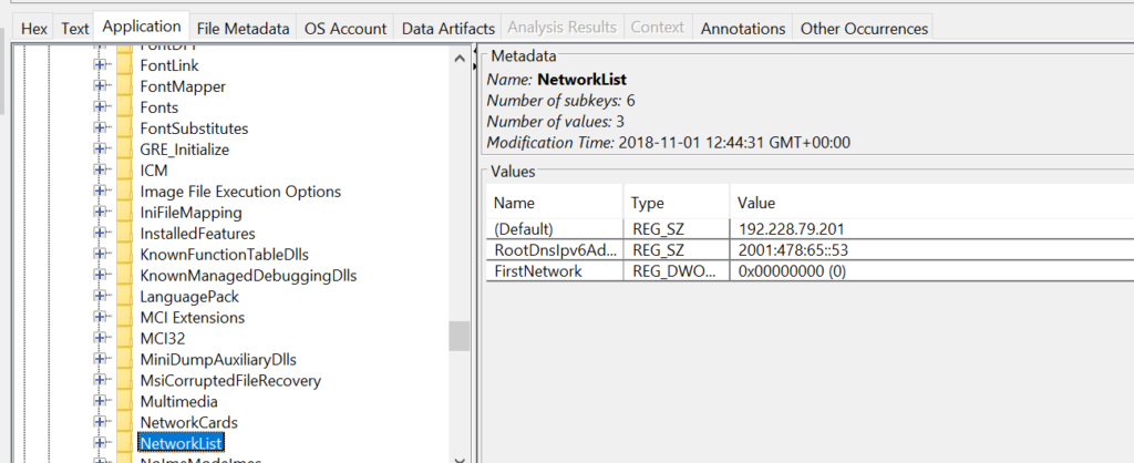
You’d use hive list commands to find registry hives in memory, which store system settings malware often tweaks these for persistence. Say you’re checking a home computer after suspicious pop-ups. This could show changes to startup keys that launch bad software every boot.

‘hivescan‘ scans for hive structures. ‘hivelist‘ lists them with virtual and physical addresses.

Volatility 2:

vol.py -f “/path/to/file” ‑‑profile <profile> hivescan

vol.py -f “/path/to/file” ‑‑profile <profile> hivelist

Volatility 3:

vol.py -f “/path/to/file” windows.registry.hivescan

vol.py -f “/path/to/file” windows.registry.hivelist

bash$ > vol -f Windows7.vmem windows.registry.hivelist

This lists the registry hives with their paths and offsets for further digging.

bash$ > vol -f Windows7.vmem windows.registry.hivescan

The scan output highlights hive locations in memory.

Printkey

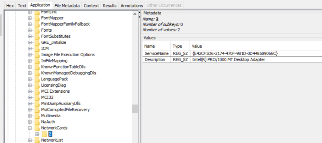
Printkey is handy for viewing specific registry keys and values, like checking for malware-added entries. For instance, in a ransomware case, you might look at keys that control file associations to see if they’ve been hijacked.

Without a key, it shows defaults, while -K or –key targets a certain path.

Volatility 2:

vol.py -f “/path/to/file” ‑‑profile <profile> printkey

vol.py -f “/path/to/file” ‑‑profile <profile> printkey -K “Software\Microsoft\Windows\CurrentVersion”

Volatility 3:

vol.py -f “/path/to/file” windows.registry.printkey

vol.py -f “/path/to/file” windows.registry.printkey ‑‑key “Software\Microsoft\Windows\CurrentVersion”

bash$ > vol -f Windows7.vmem windows.registry.printkey

This gives a broad view of registry keys.

bash$ > vol -f Windows7.vmem windows.registry.printkey –key “Software\Microsoft\Windows\CurrentVersion”

Here, it focuses on the specified key, showing subkeys and values.

Files

File Scan

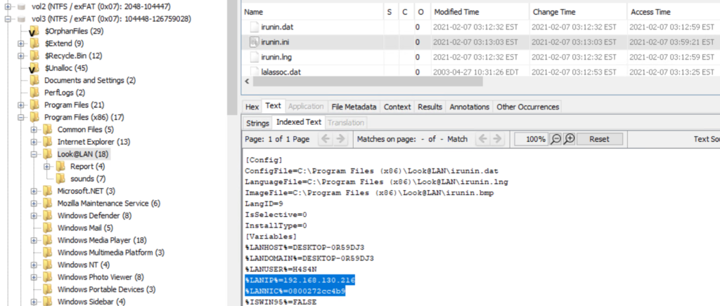
Filescan helps list files cached in memory, even deleted ones, great for finding malware files that were run but erased from disk. This can uncover temporary files from the infection.

Both versions scan for file objects in memory pools.

Volatility 2:

vol.py -f “/path/to/file” ‑‑profile <profile> filescan

Volatility 3:

vol.py -f “/path/to/file” windows.filescan

bash$ > vol -f Windows7.vmem windows.filescan

This output lists file paths, offsets, and access types.

File Dump

You’d dump files to extract them from memory for closer checks, like pulling a suspicious script. In a corporate espionage probe, dumping a hidden document could reveal leaked secrets.

Without options, it dumps all. With offsets or PID, it targets specific ones. Vol 3 uses virtual or physical addresses.

Volatility 2:

vol.py -f “/path/to/file” ‑‑profile <profile> dumpfiles ‑‑dump-dir=“/path/to/dir”

vol.py -f “/path/to/file” ‑‑profile <profile> dumpfiles ‑‑dump-dir=“/path/to/dir” -Q <offset>

vol.py -f “/path/to/file” ‑‑profile <profile> dumpfiles ‑‑dump-dir=“/path/to/dir” -p <PID>

Volatility 3:

vol.py -f “/path/to/file” -o “/path/to/dir” windows.dumpfiles

vol.py -f “/path/to/file” -o “/path/to/dir” windows.dumpfiles ‑‑virtaddr <offset>

vol.py -f “/path/to/file” -o “/path/to/dir” windows.dumpfiles ‑‑physaddr <offset>

bash$ > vol -f Windows7.vmem windows.dumpfiles

This pulls all cached files Windows has in RAM.

Miscellaneous

Malfind

Malfind scans for injected code in processes, flagging potential malware.

Vol 2 shows basics like hexdump. Vol 3 adds more details like protection and disassembly.

Volatility 2:

vol.py -f “/path/to/file” ‑‑profile <profile> malfind

Volatility 3:

vol.py -f “/path/to/file” windows.malfind

bash$ > vol -f Windows7.vmem windows.malfind

This highlights suspicious memory regions with details.

Yara Scan

Yara scan uses rules to hunt for malware patterns across memory. It’s like a custom detector. For example, during a widespread attack like WannaCry, a Yara rule could quickly find infected processes.

Vol 2 uses file path. Vol 3 allows inline rules, file, or kernel-wide scan.

Volatility 2:

vol.py -f “/path/to/file” yarascan -y “/path/to/file.yar”

Volatility 3:

vol.py -f “/path/to/file” windows.vadyarascan ‑‑yara-rules <string>

vol.py -f “/path/to/file” windows.vadyarascan ‑‑yara-file “/path/to/file.yar”

vol.py -f “/path/to/file” yarascan.yarascan ‑‑yara-file “/path/to/file.yar”

bash$ > vol -f Windows7.vmem windows.vadyarascan –yara-file yara_fules/Wannacrypt.yar

As you can see we found the malware and all related processes to it with the help of the rule

Bonus

Using the strings command, you can quickly uncover additional useful details, such as IP addresses, email addresses, and remnants from PowerShell or command prompt activities.

Emails

bash$ > strings Windows7.vmem | grep -oE "\b[A-Za-z0-9._%+-]+@[A-Za-z0-9.-]+\.[A-Za-z]{2,4}\b"

IPs

bash$ > strings Windows7.vmem | grep -oE "\b[A-Za-z0-9._%+-]+@[A-Za-z0-9.-]+\.[A-Za-z]{2,4}\b"

Powershell and CMD artifacts

bash$ > strings Windows7.vmem | grep -E "(cmd|powershell|bash)[^\s]+"

Summary

By now you should feel comfortable with all the network analysis, file dumps, hives and registries we had to go through. As you practice, your confidence will grow fast. The commands covered here will help you solve most of the cases as they are fundamental. Also, don’t forget that Volatility has a lot more different plugins that you may want to explore. Feel free to come back to this guide anytime you want. Part 1 will remind you how to approach a memory dump, while Part 2 has the commands you need. In this part, we’ve expanded your Volatility toolkit with network scans to track connections, registry tools to check settings, file commands to extract cached items, and miscellaneous scans like malfind for injections and Yara for pattern matching. Together they give you a solid set of steps. 

If you want to turn this into a career, our digital forensics courses are built to get you there. Many students use this training to prepare for industry certifications and job interviews. Our focus is on the practical skills that hiring teams look for.

Welcome back, aspiring digital forensic investigators!

The world of cybercrime continues to grow every year, and attackers constantly discover new opportunities and techniques to break into systems. One of the most dangerous and well-organized ransomware groups in recent years was Conti. Conti operated almost like a real company, with dedicated teams for developing malware, gaining network access, negotiating with victims, and even providing “customer support” for payments. The group targeted governments, hospitals, corporations, and many other high-value organizations. Their attacks included encrypting systems, stealing data, and demanding extremely high ransom payments.

For investigators, Conti became an important case study because their operations left behind a wide range of forensic evidence from custom malware samples to fast lateral movement and large-scale data theft. Even though the group officially shut down after their internal chats were leaked, many of their operators, tools, and techniques continued to appear in later attacks. This means Conti’s methods still influence modern ransomware operations which makes it a valid topic for forensic investigators.

Today, we are going to look at a ransomware incident involving Conti malware and analyze it with Splunk to understand how an Exchange server was compromised and what actions the attackers performed once inside.

Splunk

Splunk is a platform that collects and analyzes large amounts of machine data, such as logs from servers, applications, and security tools. It turns this raw information into searchable events, graphs, and alerts that help teams understand what is happening across their systems in real time. Companies mainly use Splunk for monitoring, security operations, and troubleshooting issues. Digital forensics teams also use Splunk because it can quickly pull together evidence from many sources and show patterns that would take much longer to find manually.

Time Filter

Splunk’s default time range is the last 24 hours. However, when investigating incidents, especially ransomware, you often need a much wider view. Changing the filter to “All time” helps reveal older activity that may be connected to the attack. Many ransomware operations begin weeks or even months before the final encryption stage. Keep in mind that searching all logs can be heavy on large environments, but in our case this wider view is necessary.

Index

An index in Splunk is like a storage folder where logs of a particular type are placed. For example, Windows Event Logs may go into one index, firewall logs into another, and antivirus logs into a third. When you specify an index in your search, you tell Splunk exactly where to look. But since we are investigating a ransomware incident, we want to search through every available index:

index=*

This ensures that nothing is missed and all logs across the environment are visible to us.

Fields

Fields are pieces of information extracted from each log entry, such as usernames, IP addresses, timestamps, file paths, and event IDs. They make your searches much more precise, allowing you to filter events with expressions like src_ip=10.0.0.5 or user=Administrator. In our case, we want to focus on executable files and that is the “Image”. If you don’t see it in the left pane, click “More fields” and add it.

Once you’ve added it, click Image in the left pane to see the top 10 results. 

These results are definitely not enough to begin our analysis. We can expand the list using top: 

index=* | top limit=100 Image

Here the cmd.exe process running in the Administrator’s user folder looks very suspicious. This is unusual, so we should check it closely. We also see commands like net1, net, whoami, and rundll32.

In one of our articles, we learned that net1 works like net and can be used to avoid detection in PowerShell if the security rules only look for net.exe. The rundll32 command is often used to run DLL files and is commonly misused by attackers. It seems the attacker is using normal system tools to explore the system. It also might be that the hackers used rundll32 to stay in the system longer.

At this point, we can already say the attacker performed reconnaissance and could have used rundll32 for persistence or further execution.

Hashes

Next, let’s investigate the suspicious cmd.exe more closely. Its location alone is a red flag, but checking its hashes will confirm whether it is malicious.

index=* Image="C:\\Users\\Administrator\\Documents\\cmd.exe" | table Image, Hashes

Copy one of the hashes and search for it on VirusTotal.

The results confirm that this file belongs to a Conti ransomware sample. VirusTotal provides helpful behavior analysis and detection labels that support our findings. When investigating, give it a closer look to understand exactly what happened to your system.

Net1

Now let’s see what the attacker did using the net1 command:

index=* Image=*net1.exe

The logs show that a new user was added to the Remote Desktop Users local group. This allows the attacker to log in through RDP on that specific machine. Since this is a local group modification, it affects only that workstation.

In MITRE ATT&CK, this action falls under Persistence. The hackers made sure they could connect to the host even if other credentials were lost. Also, they may have wanted to log in via GUI to explore the system more comfortably.

TargetFilename

This field usually appears in file-related logs, especially Windows Security Logs, Sysmon events, or EDR data. It tells you the exact file path and file name that a process interacted with. This can include files being created, modified, deleted, or accessed. That means we can find files that malware interacted with. If you can’t find the TargetFilename field in the left pane, just add it.

Run:

index=* Image="C:\\Users\\Administrator\\Documents\\cmd.exe"

Then select TargetFilename

We see that the ransomware created many “readme” files with a ransom note. This is common behavior for ransomware to spread notes everywhere. Encrypting data is the last step in attacks like this. We need to figure out how the attacker got into the system and gained high privileges.

Before we do that, let’s see how the ransomware was propagated across the domain:

index=* TargetFileName=*cmd.exe

While unsecapp.exe is a legitimate Microsoft binary. When it appears, it usually means something triggered WMI activity, because Windows launches unsecapp.exe only when a program needs to receive asynchronous WMI callbacks. In our case the ransomware was spread using WMI and infected other hosts where the port was open. This is a very common approach. 

Sysmon Events

Sysmon Event ID 8 indicates a CreateRemoteThread event, meaning one process created a thread inside another. This is a strong sign of malicious activity because attackers use it for process injection, privilege escalation, or credential theft.

List these events:

index=* EventCode=8

Expanding the log reveals another executable interacting with lsass.exe. This is extremely suspicious because lsass.exe stores credentials. Attacking LSASS is a common step for harvesting passwords or hashes.

Another instance of unsecapp.exe being used. It’s not normal to see it accessing lsass.exe. Our best guess here would be that something used WMI, and that WMI activity triggered code running inside unsecapp.exe that ended up touching LSASS. The goal behind it could be to dump LSASS every now and then until the domain admin credentials are found. If the domain admins are not in the Protected Users group, their credentials are stored in the memory of the machine they access. If that machine is compromised, the whole domain is compromised as well.

Exchange Server Compromise

Exchange servers are a popular target for attackers. Over the years, they have suffered from multiple critical vulnerabilities. They also hold high privileges in the domain, making them valuable entry points. In this case, the hackers used the ProxyShell vulnerability chain. The exploit abused the mailbox export function to write a malicious .aspx file (a web shell) to any folder that Exchange can access. Instead of a harmless mailbox export, Exchange unknowingly writes a web shell directly into the FrontEnd web directory. From there, the attacker can execute system commands, upload tools, and create accounts with high privileges.

To find the malicious .aspx file in our logs we should query this:

index=* source=*sysmon* *aspx

We can clearly see that the web shell was placed where Exchange has web-accessible permissions. This webshell was the access point.

Timeline

The attack began when the intruder exploited the ProxyShell vulnerabilities on the Exchange server. By abusing the mailbox export feature, they forced Exchange to write a malicious .aspx web shell into a web-accessible directory. This web shell became their entry point and allowed them to run commands directly on the server with high privileges. After gaining access, the attacker carried out quiet reconnaissance using built-in tools such as cmd.exe, net1, whoami and rundll32. Using net1, the attacker added a new user to the Remote Desktop Users group to maintain persistence and guarantee a backup login method. The attacker then spread the ransomware across the network using WMI. The appearance of unsecapp.exe showed that WMI activity was being used to launch the malware on other hosts. Sysmon Event ID 8 logged remote thread creation where the system binary attempts to access lsass.exe. This suggests the attacker tried to dump credentials from memory. This activity points to a mix of WMI abuse and process injection aimed at obtaining higher privileges, especially domain-level credentials. 

Finally, once the attacker had moved laterally and prepared the environment, the ransomware (cmd.exe) encrypted systems and began creating ransom note files throughout these systems. This marked the last stage of the operation.

Summary

Ransomware is more than just a virus, it’s a carefully planned attack where attackers move through a network quietly before causing damage. In digital forensics we often face these attacks and investigating them means piecing together how it entered the system, what tools it used, which accounts it compromised, and how it spread. Logs, processes, file changes tell part of the story. By following these traces, we understand the attacker’s methods, see where defenses failed, and learn how to prevent future attacks. It’s like reconstructing a crime scene. Sometimes, we might be lucky enough to shut down their entire infrastructure before they can cause more damage.

If you need forensic assistance, you can hire our team to investigate and mitigate incidents. Additionally, we provide classes on digital forensics for those looking to expand their skills and understanding in this field. 

Welcome back, aspiring digital forensics investigators!

In the previous article we introduced Autopsy and noted its wide adoption by law enforcement, federal agencies and other investigative teams. Autopsy is a forensic platform built on The Sleuth Kit and maintained by commercial and community contributors, including the Department of Homeland Security. It packages many common forensic functions into one interface and automates many of the repetitive tasks you would otherwise perform manually.

Today, let’s focus on Autopsy and how we can investigate a simple case with the help of this app. We will skip the basics as we have previously covered it. 

Analysis

Artifacts and Evidence Handling

Start from the files you are given. In this walkthrough we received an E01 file, which is the EnCase evidence file format. An E01 is a forensic image container that stores a sector-by-sector copy of a drive together with case metadata, checksums and optional compression or segmentation. It is a common format in forensic workflows and preserves the information needed to verify later that an image has not been altered.

Before any analysis begins, confirm that your working copy matches the original by comparing hash values. Tools used to create forensic images, such as FTK Imager, normally generate a short text report in the same folder that lists the image metadata and hashes you can use for verification.

Autopsy also displays the same hash values once the image is loaded. To see that select the Data Source and view the Summary in the results pane to confirm checksums and metadata.

Enter all receipts and transfers into the chain of custody log. These records are essential if your findings must be presented in court.

Opening Images In Autopsy

Create a new case and add the data source. If you have multiple EnCase segments in the same directory, point Autopsy to the first file and it will usually pick up the remaining segments automatically. Let the ingest modules run as required for your investigative goals, and keep notes about which modules and keyword searches you used so your process is reproducible.

Identifying The Host

First let’s see the computer name we are looking at. Names and labelling conventions can differ from the actual system name recorded in the image. You can quickly find the host name listed under Operating System Information, next to the SYSTEM entry. 

Knowing the host name early helps orient the rest of your analysis and simplifies cross-referencing with network or domain logs.

Last Logins and User Activity

To understand who accessed the machine and when, we can review last login and account activity artifacts. Windows records many actions in different locations. These logs are extremely useful but also mean attackers sometimes attempt to use those logs to their own advantage. For instance, after a domain compromise an attacker can review all security logs and find machines that domain admins frequently visit. It doesn’t take much time to find out what your critical infrastructure is and where it is located with the help of such logs. 

In Autopsy, review Operating System, then User Accounts and sort by last accessed or last logon time to see recent activity. Below we see that Sivapriya was the last one to login.

A last logon alone does not prove culpability. Attackers may act during normal working hours to blend in, and one user’s credentials can be used by another actor. You need to use time correlation and additional artifacts before drawing conclusions.

Installed Applications

Review installed applications and files on the system. Attackers often leave tools such as Python, credential dumpers or reconnaissance utilities on disk. Some are portable and will be found in Temp, Public or user directories rather than in Program Files. Execution evidence can be recovered from Prefetch, NTUSER.DAT, UserAssist, scheduled tasks, event logs and other sources we will cover separately.

In this case we found a network reconnaissance tool, Look@LAN, which is commonly used for mapping local networks.

Signed and legitimate tools are sometimes abused because they follow expected patterns and can evade simple detection.

Network Information and IP Addresses

Finding the IP address assigned to the host is useful for reconstructing lateral movement and correlating events across machines and the domain controller. The domain controller logs validate domain logons and are essential for tracing where an attacker moved next. In the image you can find network assignments in registry hives: the SYSTEM hive contains TCP/IP interface parameters under CurrentControlSet\Services\Tcpip\Parameters\Interfaces and Parameters, and the SOFTWARE hive stores network profile signatures under Microsoft\Windows NT\CurrentVersion\NetworkList\Signatures\Managed and \Unmanaged or NetworkList

If the host used DHCP, registry entries may show previously assigned IPs, but sometimes the attacker’s tools carry their own configuration files. In our investigation we inspected an application configuration file (irunin.ini) found in Program Files (x86) and recovered the IP and MAC address active when that tool was executed. 

The network adapter name and related entries are also recorded under SOFTWARE\Microsoft\Windows NT\CurrentVersion\NetworkCards.

User Folders and Files

Examine the Users folder thoroughly. Attackers may intentionally store tools and scripts in other directories to create false flags, so check all profiles, temporary locations and shared folders. When you extract an artifact for analysis, hash it before and after processing to demonstrate integrity. In this case we located a PowerShell script that attempts privilege escalation.

The script checks if it is running as an administrator. If elevated it writes the output of whoami /all to %ALLUSERSPROFILE%\diag\exec_<id>.dat. If not elevated, it temporarily sets a value under HKCU\Environment\ProcExec with a PowerShell launch string, then triggers the built-in scheduled task \Microsoft\Windows\DiskCleanup\SilentCleanup via schtasks /run in the hope that the privileged task will pick up and execute the planted command, and finally removes the registry value. Errors are logged to a temporary diag file.

The goal was to validate a privilege escalation path by causing a higher-privilege process to run a payload and record the resulting elevated identity.

Credential Harvesting

We also found evidence of credential dumping tools in user directories. Mimikatz was present in Hasan’s folder, and Lazagne was also detected in Defender logs. These tools are commonly used to extract credentials that support lateral movement. The presence of python-3.9.1-amd64.exe in the same folder suggests the workstation could have been used to stage additional tools or scripts for propagation.

Remember that with sufficient privileges an attacker can place malicious files into other users’ directories, so initial attribution based only on file location is tentative.

Windows Defender and Detection History

If endpoint protection was active, its detection history can hold valuable context about what was observed and when. Windows Defender records detection entries can be found under C:\ProgramData\Microsoft\Windows Defender\Scans\History\Service\DetectionHistory*. 
Below we found another commonly used tool called LaZagne, which is available for both Linux and Windows and is used to extract credentials. Previously, we have covered the use of this tool a couple of times and you can refer to Powershell for Hackers – Basics to see how it works on Windows machines.

Correlate those entries with file timestamps, prefetch data and event logs to build a timeline of execution.

Zerologon

It was also mentioned that the attackers attempted the Zerologon exploit. Zerologon (CVE-2020-1472) is a critical vulnerability in the Netlogon protocol that can allow an unauthenticated attacker with network access to a domain controller to manipulate the Netlogon authentication process, potentially resetting a computer account password and enabling impersonation of the domain controller. Successful exploitation can lead to domain takeover. 

Using keyword searches across the drive we can find related files, logs and strings that mention zerologon to verify any claims. 

In the image above you can see NTUSER.DAT contains “Zerologon”. NTUSER.DAT is the per-user registry hive stored in each profile and is invaluable for forensics. It contains persistent traces such as Run and RunOnce entries, recently opened files and MRU lists, UserAssist, TypedURLs data, shells and a lot more. The presence of entries in a user’s NTUSER.DAT means that the user’s account environment recorded those actions. The entry appears in Sandhya’s NTUSER.DAT in this case, it suggests that the account participated in this activity or that artifacts were created while that profile was loaded.

Timeline

Pulling together the available artifacts suggests the following sequence. The first login on the workstation appears to have been by Sandhya, during which a Zerologon exploit was attempted but failed. After that, Hasan logged in and used tools to dump credentials, possibly to start moving laterally. Evidence of Mimikatz and a Python installer were found in Hasan’s directory. Finally, Sivapriya made the last recorded login on this workstation and a PowerShell script intended to escalate privileges was found in their directory. This script could have been used during lateral activity to escalate privileges on other hosts or if local admin rights were not assigned to Hasan, another attacker could have tried to escalate their privileges using Sivapriya’s account. At this stage it is not clear whether multiple accounts represent separate actors working together or a single hacker using different credentials. Resolving that requires cross-host correlation, domain controller logs and network telemetry.

Next Steps and Verification

This was a basic Autopsy workflow. For stronger attribution and a complete reconstruction we need to collect domain controller logs, firewall and proxy logs and any endpoint telemetry available. Specialised tools can be used for deeper analysis where appropriate.

Conclusion

As you can see, Autopsy is an extensible platform that can organize many routine forensic tasks, but it is only one part of a comprehensive investigation. Successful disk analysis depends on careful evidence handling and multiple data sources. It’s also important to confirm hashes and chain of custody before and after the analysis. When you combine solid on-disk analysis with domain and network logs, you can move from isolated observations to a defensible timeline and conclusions. 

If you need forensic assistance, we offer professional services to help investigate and mitigate incidents. Additionally, we provide classes on digital forensics for those looking to expand their skills and understanding in this field.

Welcome back, aspiring digital forensic analysts!

There are times when our work requires repairing damaged disks to perform a proper forensic analysis. Attackers use a range of techniques to cover their tracks. These can be corrupting the boot sector, overwriting metadata, physically damaging a drive, or exposing hardware to high heat. That’s what they did in Mr.Robot. 

Physical damage often destroys data beyond practical recovery, but a much more common tactic is logical sabotage. Attackers wipe partitions, corrupt the Master Boot Record, or otherwise tamper with the file system to slow or confuse investigators. Most real-world incidents that require disk-level recovery come from remote activity rather than physical tampering, unless the case involves an insider with physical access to servers or workstations.

Inexperienced administrators sometimes assume that data becomes irrecoverable after tampering, or that simply deleting files destroys their content and structure. That is not true. In this article we will examine how disks can be repaired and how deleted files can still be discovered and analysed.

In our previous article, PowerShell for Hackers: Mayhem Edition, we showed how an attacker can overwrite the MBR and render Windows unbootable. Today we will examine an image with a deliberately damaged boot sector. The machine that produced the image was used for data exfiltration. An insider opened an important PDF that contained a canary token and that token notified the owner that the document had been opened. It also showed the host that was used to access the file. Everything else is unknown and we will work through the evidence together.

Fixing the Drive

Corrupting the disk boot sector is straightforward in principle. You alter the data the system expects to find there so the OS cannot load the disk in the normal way. File formats, executables, archives, images and other files have internal headers and structures that tell software how to interpret their contents. Changing a file extension does not change those internal headers, so renaming alone is a poor method of concealment. Tools that inspect file headers and signatures will still identify the real file type. Users sometimes try to hide VeraCrypt containers by renaming them to appear as ordinary executables. Forensic tools and signature scanners will still flag such anomalies. Windows also leaves numerous artefacts that can indicate which files were opened. Among them are MRU lists, Jump Lists, Recent Items and other traces created by common applications, including simple editors.

Before we continue, let’s see what evidence we were given.

Above is a forensic image and below is a text file with metadata about that image. As a forensic analyst you should verify the integrity of the evidence by comparing the computed hash of the image with the hash recorded in the metadata file.

If the hash matches, work only on a duplicate and keep the original evidence sealed. Create a verified working copy for all further analysis.

Opening a disk image with a corrupted boot sector in Autopsy or FTK Imager will not succeed, as many of these tools expect a valid partition table and a readable boot sector. In such cases you will need to repair the image manually with a hex editor such as HxD so other tools can parse the structure.

The first 512 bytes of a disk image contain the MBR (Master Boot Record) on traditional MBR-partitioned media. In this image the final two bytes of that sector were modified. A valid MBR should end with the boot signature 0x55 0xAA. Those two bytes tell the firmware and many tools that the sector contains a valid boot record. Without the signature the image may be unreadable, so restoring the correct 0x55AA signature is the first step we need to do. 

When editing the MBR in a hex editor, do not delete bytes with backspace, you need to overwrite them. Place the cursor before the bytes to be changed and type the new hex values. The editor will replace the existing bytes without shifting the file.

Partitions

This image contains two partitions. In a hex view you can see the partition table entries that describe those partitions. In forensic viewers such as FTK Imager and Autopsy those partitions will be displayed graphically once the MBR and partition table are valid.

Both of them are in the black frame. The partition table entries also encode the partition size and starting sector in little-endian form, which requires byte-order interpretation and calculation to convert to human-readable sizes. For example, if you see an entry that corresponds to 63,401,984 sectors and each sector is 512 bytes, the size calculation is:

63,401,984 sectors × 512 bytes = 32,461,815,808 bytes, which is 32.46 GB (decimal) or ≈ 30.23 GiB

FTK Imager

Now let’s use FTK Imager to view the contents of our evidence file. In FTK Imager choose File, then Add Evidence Item, select Image File, and point the application to the verified copy of the image.

Once the MBR has been repaired and the image loaded, FTK Imager will display the partitions and expose their file systems. While Autopsy and other automated tools can handle a large portion of the analysis and save time, manual inspection gives you a deeper understanding of how Windows stores metadata and how to validate automated results. In this article we will show how to manually get the results and put the results together using Zimmer’s forensic utilities.

$MFT

Our next goal is to analyse the $MFT (Master File Table). The $MFT is a special system file on NTFS volumes that acts as an index for every file and directory on the file system. It contains records with metadata about filenames, timestamps, attributes, and, in many cases, pointers to file data. The $MFT is hidden in File Explorer, but it is always present on NTFS volumes (for example, C:$MFT)

Export the $MFT from the mounted or imaged volume. Right-click the $MFT entry in your forensic viewer and choose Export Files

To parse and extract readable output from the $MFT you can use MFTECmd.exe, a tool included in Eric Zimmerman’s EZTools collection. From a command shell run the extractor, for example:

PS> MFTECmd.exe -f ..\Evidence$MFT --csv ..\Evidence\ --csvf MFT.csv

The command above creates a CSV file you can use for keyword searches and timeline work. If needed, rename the exported files to make it easier to work with them in PowerShell.

When a CSV file is opened, you can use basic keyword search or pick an extension to see what files existed on the drive. 

Understanding and working with $MFT records is important. If a suspect deleted a file, the $MFT may still contain its last known filename, path, timestamps and sometimes even data pointers. That information lets investigators target data recovery and build a timeline of the suspect’s activity.

Suspicious Files

During inspection of the second partition we located several suspicious entries. Many were marked as deleted but can still be exported and examined.

The evidence shows the perpetrator had a utility named DiskWipe.exe, which suggests an attempt to remove traces. We also found references to sensitive corporate documents, which together indicates data exfiltration. At this stage we can confirm the machine was used to access sensitive files. If we decide to analyze further, we can use registry and disk data to see whether the wiping utility was actually executed and what user executed it. This is outside of our scope today.

$USNJRNL

The $USNJRNL (Update Sequence Number Journal) is another hidden NTFS system file that records changes to files and directories. It logs actions such as creation, modification and deletion before those actions are committed to disk. Because it records a history of file-system operations, $UsnJrnl ($J) can be invaluable in cases involving mass file deletion or tampering. 

To extract the journal, first go to root, then $Extend and double-click $UsnJrnl. You need a $J file.

You can then parse it with MFTECmd in the same way:

PS> MFTECmd.exe -f ..\Evidence$J --csv ..\Evidence\ --csvf J.csv

Since the second partition had the wiper, we can assume the perpetrator deleted files to cover traces. Let’s open the CSV in Timeline Explorer and set the Update Reason to FileDelete to view deleted files.

Among the deleted entries we found a folder named “data Exfil.” In many insider exfiltration cases the perpetrator will compress those folders before transfer, so we searched $MFT and $J for archive extensions. Multiple entries for files named “New Compressed (zipped) Folder.zip” were present.

The journal shows the zip was created and files were appended to it. The final operation was a rename (RenameOldName). Using the Parent Entry Number exposed in $J we can correlate entries and recover the original folder name.

As you can see, using the Parent Entry Number we found that the original folder name was “data Exfil” which was later deleted by the suspect.

Timeline

From the assembled artifacts we can conclude that the machine was used to access and exfiltrate sensitive material. We found Excel sheets, PDFs, text documents and zip archives with sensitive data. The insider created a folder called “data Exfil,” packed its contents into an archive, and then attempted to cover tracks using a wiper. DiskWipe.exe and the deleted file entries support our hypothesis. To confirm execution and attribute actions to a user, we can examine registry entries, prefetch files, Windows event logs, shellbags and user profile activity that may show us process execution and the account responsible for it. The corrupted MBR suggests the perpetrator also intentionally damaged the boot sector to complicate inspection.

Summary

Digital forensics is a fascinating field. It exposes how much information an operating system preserves about user actions and how those artifacts can be used to reconstruct events. Many Windows features were designed to improve reliability and user experience, but those same features give us useful forensic traces. Although automated tools can speed up analysis, skilled analysts must validate tool output by understanding the underlying data structures and by performing manual checks when necessary. As you gain experience with the $MFT, $UsnJrnl and low-level disk structures, you will become more effective at recovering evidence and validating your hypotheses. See you soon!

Welcome back, aspiring SCADA hackers!

Today we introduce some of the most popular SCADA / ICS protocols that you will encounter during forensic investigations, incident response and penetration tests. Mastering SCADA forensics is an important career step for anyone focused on industrial cybersecurity. Understanding protocol behavior, engineering workflows, and device artifacts is a skill that employers in utilities, manufacturing, oil & gas, and building automation actively seek. Skilled SCADA forensic analysts can extract evidence with protocol fluency to perform analysis and translate findings into recommendations.

In our coming course in November on SCADA Forensics we will be using realistic ICS network topologies and simulated attacks on devices like PLCs and RTUs. You will reconstruct attack chains, identify indicators of compromise (IOCs) and analyze artifacts across field devices, engineering workstations, and HMI systems. All of that will make your profile unique.

Let’s learn about some popular protocols in SCADA environments.

Modbus

Modbus was developed in 1979 by Modicon as a simple master/slave protocol for programmable logic controllers (PLCs). It became an open standard because it was simple, publicly documented and royalty-free. Now it exists in two main flavors such as serial (Modbus RTU) and Modbus TCP. You’ll find it everywhere in legacy industrial equipment, like PLC I/O, sensors, RTUs and in small-to-medium industrial installations where simplicity and interoperability matter. Because it’s simple and widespread, Modbus is a frequent target for security research and forensic analysis.

DNP3

DNP3 (Distributed Network Protocol) originated in the early 1990s and was developed to meet the tougher telemetry needs of electric utilities. It was later standardized by IEEE. Today DNP3 is strong in electric, water and other utility SCADA systems. It supports features for telemetry, like timestamped events, buffered event reporting and was designed for unreliable or noisy links, which makes it ideal for remote substations and field RTUs. Modern deployments often run DNP3 over IP and may use the secure encrypted variants.

IEC 60870 (especially IEC 60870-5-104)

IEC 60870 is a family of telecontrol standards created for electric power system control and teleprotection. The 60870-5-104 profile (commonly called IEC 104) maps those telecontrol services onto TCP/IP. It is widely used in Europe and regions following IEC standards, so expect it in European grids and many vendor products that target telecom-grade reliability.

Malware can “speak” SCADA/ICS protocols too. For instance, Industroyer (also known as CrashOverride) that was used in the second major cyberattack on Ukraine’s power grid on December 17, 2016, by the Russian-linked Sandworm group had built-in support for multiple industrial control protocols like IEC 61850, IEC 104, OLE for Process Control Data Access (OPC DA), and DNP3. Essentially it used protocol languages to directly manipulate substations, circuit breakers, and other grid hardware without needing deeper system access.

EtherNet/IP (EIP / ETHERNET_IP)

EtherNet/IP adapts the Common Industrial Protocol (CIP) to standard Ethernet. Developed in the 1990s and standardized through ODVA, it brought CIP services to TCP/UDP over Ethernet. Now it’s widespread in manufacturing and process automation, especially in North America. It supports configuration and file transfers over TCP and I/O, cyclic data over UDP, using standard ports (TCP 44818). You’ll see it on plant-floor Ethernet networks connecting PLCs, I/O modules, HMIs and drives. 

S7 (Siemens S7 / S7comm)

S7comm (Step 7 communications) is Siemens’ proprietary protocol family used for the SIMATIC S7 PLC series since the 1990s. It is tightly associated with Siemens PLCs and the Step7 / TIA engineering ecosystem. Today it is extremely common where Siemens PLCs are deployed. Mainly in manufacturing, process control and utilities. S7 traffic often includes programs for device diagnostics, so that makes it high-value for both legitimate engineering and hackers. S7-based communications can run over Industrial Ethernet or other fieldbuses.

BACnet

BACnet (Building Automation and Control Network) was developed through ASHRAE and became ANSI/ASHRAE Standard 135 in the 1990s. It’s the open standard for building automation. Now BACnet is used in building management systems, such as HVAC, lighting, access control, fire systems and other building services. You’ll see BACnet on wired (BACnet/IP and BACnet MSTP) and wireless links inside commercial buildings, and it’s a key protocol to know when investigating building-level automation incidents.

HART-IP

HART started as a hybrid analog/digital field instrument protocol (HART) and later evolved to include HART-IP for TCP/IP-based access to HART device data. The FieldComm Group maintains HART standards. The protocol brings process instrumentation like valves, flow meters, transmitters onto IP networks so instrument diagnostics and configuration can be accessed from enterprise or control networks. It’s common in process industries, like oil & gas, chemical and petrochemical.

EtherCAT

EtherCAT (Ethernet for Control Automation Technology) is a real-time Ethernet protocol standardized under IEC 61158 and maintained by the EtherCAT Technology Group. It introduced “processing on the fly” for very low latency. It is frequent in motion control, robotics, and high-speed automation where deterministic, very low-latency communication is required. You’ll find it in machine tools, robotics cells and applications that require precise synchronization.

POWERLINK (Ethernet POWERLINK / EPL)

Ethernet POWERLINK emerged in the early 2000s as an open real-time Ethernet profile for deterministic communication. It’s managed historically by the EPSG and adopted by several vendors. POWERLINK provides deterministic cycles and tight synchronization for motion and automation tasks. Can be used in robotics, drives, and motion-critical machine control. It’s one of the real-time Ethernet families alongside EtherCAT, PROFINET-IRT and others.

Summary

We hope you found this introduction both clear and practical. SCADA protocols are the backbone of industrial operations and each one carries the fingerprints of how control systems communicate, fail, and recover. Understanding these protocols is important to carry out investigations. Interpreting Modbus commands, DNP3 events, or S7 traffic can help you retrace the steps of an attacker or engineer precisely.

In the upcoming SCADA Forensics course, you’ll build on this foundation and analyze artifacts across field devices, engineering workstations, and HMI systems. These skills are applicable in defensive operations, threat hunting, industrial digital forensics and industrial incident response. You will know how to explain what happened and how to prevent it. In a field where reliability and safety are everything, that kind of expertise can generate a lot of income.

See you there!

Learn more: https://hackersarise.thinkific.com/courses/scada-forensics

The post SCADA (ICS) Hacking and Security: SCADA Protocols and Their Purpose first appeared on Hackers Arise.

Welcome back, aspiring DFIR investigators!

If you’re diving into digital forensics, memory analysis is one of the most exciting and useful skills you can pick up. Essentially, you take a snapshot of what’s happening inside a computer’s brain right at that moment and analyze it. Unlike checking files on a hard drive, which shows what was saved before, memory tells you about live actions. Things like running programs or hidden threats that might disappear when the machine shuts down. This makes it super helpful for solving cyber incidents, especially when bad guys try to cover their tracks.

In this guide, we’re starting with the basics of memory analysis using a tool called Volatility. We’ll cover why it’s so important, how to get started, and some key commands to make you feel confident. This is part one, where we focus on the foundations and give instructions. Stick around for part two, where we’ll keep exploring Volatility and dive into network details, registry keys, files, and scans like malfind and Yara rules. Plus, if you make it through part two, there are some bonuses waiting to help you extract even more insights quickly.

Memory Forensics

Memory analysis captures stuff that disk forensics might miss. For example, after a cyber attack, malware could delete its own files or run without saving anything to the disk at all. That leaves you with nothing to find on the hard drive. But in memory, you can spot remnants like active connections or secret codes. Even law enforcement grabs memory dumps from suspects’ computers before powering them off. Once it’s off, the RAM clears out, and booting back up might be tricky if the hacker sets traps. Hackers often use tricks like USB drives that trigger wipes of sensitive data on shutdown, cleaning everything in seconds so authorities find nothing. We’re not diving into those tricks here, but they show why memory comes first in many investigations.

Lucky for us, Volatility makes working with these memory captures straightforward. It started evolving, and in 2019, Volatility 3 arrived with better syntax and easier to remember commands. We’ll look at both Volatility 2 and 3, sharing commands to get you comfortable. These should cover what most analysts need.

Memory Gems

Below is some valuable data you can find in RAM for investigations:

1. Network connections

2. File handles and open files

3. Open registry keys

4. Running processes on the system

5. Loaded modules

6. Loaded device drivers

7. Command history and console sessions

8. Kernel data structures

9. User and credential information

10. Malware artifacts

11. System configuration

12. Process memory regions

Keep in mind, sometimes key data like encryption keys hides in memory. Memory forensics can pull this out, which might be a game-changer for a case.

Approach to Memory Forensics

In this section we will describe a structured method for conducting memory forensics, designed to support investigations of data in memory. It is based on the six-step process from SANS for analyzing memory.

Identifying and Checking Processes

Start by listing all processes that are currently running. Harmful programs can pretend to be normal ones, often using names that are very similar to trick people. To handle this:

1. List every active process.

2. Find out where each one comes from in the operating system.

3. Compare them to lists of known safe processes.

4. Note any differences or odd names that stand out.

Examining Process Details

After spotting processes that might be problematic, look closely at the related dynamic link libraries (DLLs) and resources they use. Bad software can hide by misusing DLLs. Key steps include:

1. Review the DLLs connected to the questionable process.

2. Look for any that are not approved or seem harmful.

3. Check for evidence of DLLs being inserted or taken over improperly.

Reviewing Network Connections

A lot of malware needs to connect to the internet, such as to contact control servers or send out stolen information. To find these activities:

1. Check the open and closed network links stored in memory.

2. Record any outside IP addresses and related web domains.

3. Figure out what the connection is for and why it’s happening.

4. Confirm if the process is genuine.

5. See if it usually needs network access.

6. Track it back to the process that started it.

7. Judge if its actions make sense.

Finding Code Injection

Skilled attackers may use methods like replacing a process’s code or working in hidden memory areas. To detect this:

1. Apply tools for memory analysis to spot unusual patterns or signs of these tactics.

2. Point out processes that use strange memory locations or act in unexpected ways.

Detecting Rootkits

Attackers often aim for long-term access and hiding. Rootkits bury themselves deep in the system, giving high-level control while staying out of sight. To address them:

1. Search for indicators of rootkit presence or major changes to the OS.

2. Spot any processes or drivers with extra privileges or hidden traits.

Isolating Suspicious Items

Once suspicious processes, drivers, or files are identified, pull them out for further study. This means:

1. Extract the questionable parts from memory.

2. Save them safely for detailed review with forensic software.

The Volatility Framework

A widely recommended option for memory forensics is Volatility. This is a prominent open-source framework used in the field. Its main component is a Python script called Volatility, which relies on various plugins to carefully analyze memory dumps. Since it is built on Python, it can run on any system that supports Python.

Volatility’s modules, also known as plugins, are additional features that expand the framework’s capabilities. They help pull out particular details or carry out targeted examinations on memory files.

Frequently Used Volatility Modules

Here are some modules that are often used:

pslist: Shows the active processes.

cmdline: Reveals the command-line parameters for processes.

netscan: Checks for network links and available ports.

malfind: Looks for possible harmful code added to processes.

handles: Examines open resources.

svcscan: Displays services in Windows.

dlllist: Lists the dynamic-link libraries loaded in a process.

hivelist: Identifies registry hives stored in memory.

You can find documentation on Volatility here:

Volatility v2: https://github.com/volatilityfoundation/volatility/wiki/Command-Reference

Volatility v3: https://volatility3.readthedocs.io/en/latest/index.html

Installation

Installing Volatility 3 is quite easy and will require a separate virtual environment to keep things organized. Create it first before proceeding with the rest:

bash$ > python3 -m venv ~/venvs/vol3

bash$ > source ~/venvs/vol3

Now you are ready to install it:

bash$ > pip install volatility3

Since we are going to cover Yara rules in Part 2, we will need to install some dependencies:

bash$ > sudo apt install -y build-essential pkg-config libtool automake libpcre3-dev libjansson-dev libssl-dev libyara-dev python3-dev

bash$ > pip install yara-python pycryptodome

Yara rules are important and they help you automate half the analysis. There are hundreds of these rules available on Github, so you can download and use them each time you analyze the dump. While these rules can find a lot of things, there is always a chance that malware can fly under the radar, as attackers change tactics and rewrite payloads. 

Now we are ready to work with Volatility 3.

Plugins

Volatility comes with multiple plugins. To list all the available plugins do this:

bash$ > vol -h

Each of these plugins has a separate help menu with a description of what it does.

Memory Analysis Cheat Sheet

Image Information

Imagine you’re an analyst investigating a hacked computer. You start with image information because it tells you basics like the OS version and architecture. This helps Volatility pick the right settings to read the memory dump correctly. Without it, your analysis could go wrong. For example, if a company got hit by ransomware, knowing the exact Windows version from the dump lets you spot if the malware targeted a specific weakness.

In Volatility 2, ‘imageinfo‘ scans for profiles, and ‘kdbgscan‘ digs deeper for kernel debug info if needed. Volatility 3’s ‘windows.info‘ combines this, showing 32/64-bit, OS versions, and kernel details all in one and it’s quicker.

bash$ > vol -f Windows.vmem windows.info

Here’s what the output looks like, showing key system details to guide your next steps.

Process Information

As a beginner analyst, you’d run process commands to list what’s running on the system, like spotting a fake “explorer.exe” that might be malware stealing data. Say you’re checking a bank employee’s machine after a phishing attack, these commands can tell you if suspicious programs are active, and help you trace the breach.

‘pslist‘ shows active processes via kernel structures. ‘psscan‘ scans memory for hidden ones (good for rootkits). ‘pstree‘ displays parent-child relationships like a family tree. ‘psxview‘ in Vol 2 compares lists to find hidden processes.

Note that Volatility 2 wants you to specify the profile. You can find out the profile while gathering the image info.

Volatility 2:

vol.py -f “/path/to/file” ‑‑profile <profile> pslist

vol.py -f “/path/to/file” ‑‑profile <profile> psscan

vol.py -f “/path/to/file” ‑‑profile <profile> pstree

vol.py -f “/path/to/file” ‑‑profile <profile> psxview

Volatility 3:

vol.py -f “/path/to/file” windows.pslist

vol.py -f “/path/to/file” windows.psscan

vol.py -f “/path/to/file” windows.pstree

Now let’s see what we get:

bash$ > vol -f Windows7.vmem windows.pslist

This output lists processes with PIDs, names, and start times. Great for spotting outliers.

bash$ > vol -f Windows.vmem windows.psscan

Here, you’ll see a broader scan that might catch processes trying to hide.

bash$ > vol -f Windows7.vmem windows.pstree

This tree view helps trace how processes relate, like if a browser spawned something shady.

Displaying the entire process tree will look messy, so we recommend a more targeted approach with –pid

Process Dump

You’d use process dump when you spot a suspicious process and want to extract its executable for closer inspection, like with antivirus tools. For instance, if you’re analyzing a system after a data leak, dumping a weird process could reveal it is spyware sending info to hackers.

Vol 2’s ‘procdump‘ pulls the exe for a PID. Vol 3’s ‘dumpfiles‘ grabs the exe plus related DLLs, giving more context.

Volatility 2:

vol.py -f “/path/to/file” ‑‑profile <profile> procdump -p <PID> ‑‑dump-dir=“/path/to/dir”

Volatility 3:

vol.py -f “/path/to/file” -o “/path/to/dir” windows.dumpfiles ‑‑pid <PID>

We already have a process we are interested in:

bash$ > vol -f Windows.vmem windows.dumpfiles --pid 504

After the dump, check the output and analyze it further.

Memdump

Memdump is key for pulling the full memory of a process, which might hold passwords or code snippets. Imagine investigating insider theft, dumping memory from an email app could show unsent drafts with stolen data.

Vol 2’s ‘memdump’ extracts raw memory for a PID. Vol 3’s ‘memmap’ with –dump maps and dumps regions, useful for detailed forensics.

Volatility 2:

vol.py -f “/path/to/file” ‑‑profile <profile> memdump -p <PID> ‑‑dump-dir=“/path/to/dir”

Volatility 3:

vol.py -f “/path/to/file” -o “/path/to/dir” windows.memmap ‑‑dump ‑‑pid <PID>

Let’s see the output for our process:

bash$ > vol -f Windows7.vmem windows.memmap --dump --pid 504

This shows the memory map and dumps files for deep dives.

DLLs

Listing DLLs helps spot injected code, like malware hiding in legit processes. Unusual DLLs might point to infection.

Both versions list loaded DLLs for a PID, but Vol 3 is profile-free and faster.

Volatility 2:

vol.py -f “/path/to/file” ‑‑profile <profile> dlllist -p <PID>

Volatility 3:

vol.py -f “/path/to/file” windows.dlllist ‑‑pid <PID>

Let’s see the DLLs loaded in our memory dump:

bash$ > vol -f Windows7.vmem windows.dlllist --pid 504

Here you see all loaded DLLs of this process. You already know how to dump processes with their DLLs for a more thorough analysis. 

Handles

Handles show what a process is accessing, like files or keys crucial for seeing if malware is tampering with system parts. In a ransomware case, handles might reveal encrypted files being held open or encryption keys used to encrypt data.

Both commands list handles for a PID. Similar outputs, but Vol 3 is streamlined.

Volatility 2:

vol.py -f “/path/to/file” ‑‑profile <profile> handles -p <PID>

Volatility 3:

vol.py -f “/path/to/file” windows.handles ‑‑pid <PID>

Let’s see the handles our process used:

bash$ > vol -f Windows.vmem windows.handles --pid 504

It gave us details, types and names for clues.

Services

Services scan lists background programs, helping find persistent malware disguised as services. If you’re probing a server breach, this could uncover a backdoor service.

Use | more to page through long lists. Outputs are similar, showing service names and states.

Volatility 2:

vol -f “/path/to/file” ‑‑profile <profile> svcscan | more

Volatility 3:

vol -f “/path/to/file”  windows.svcscan | more

Since this technique is often abused, a lot can be discovered here:

bash$ > vol -f Windows7.vmem windows.svcscan

Give it a closer look and spend enough time here. It’s good to familiarize yourself with native services and their locations

Summary

We’ve covered the essentials of memory analysis with Volatility, from why it’s vital to key commands for processes, dumps, DLLs, handles, and services. Apart from the commands, now you know how to approach memory forensics and what actions you should take. As we progress, more articles will be coming where we practice with different cases. We already have a memory dump of a machine that suffered a ransomware attack, which we analyzed with you recently. In part two, you will build on this knowledge by exploring network info, registry, files, and advanced scans like malfind and Yara rules. And for those who finish part two, some handy bonuses await to speed up your work even more. Stay tuned!

The post Digital Forensics: Volatility – Memory Analysis Guide, Part 1 first appeared on Hackers Arise.

Welcome back, my aspiring SCADA/ICS cyberwarriors!

SCADA (Supervisory Control and Data Acquisition) systems and the wider class of industrial control systems (ICS) run many parts of modern life, such as electricity, water, transport, factories. These systems were originally built to work in closed environments and not to be exposed to the public Internet. Over the last decade they have been connected more and more to corporate networks and remote services to improve efficiency and monitoring. That change has also made them reachable by the same attackers who target regular IT systems. When a SCADA system is hit by malware, sabotage, or human error, operators must restore service fast. At the same time investigators need trustworthy evidence to find out what happened and to support legal, regulatory, or insurance processes.

Forensics techniques from traditional IT are helpful, but they usually do not fit SCADA devices directly. Many field controllers run custom or minimal operating systems, lack detailed logs, and expose few of the standard interfaces that desktop forensics relies on. To address that gap, we are starting a focused, practical 3-day course on SCADA forensics. The course is designed to equip you with hands-on skills for collecting, preserving and analysing evidence from PLCs, RTUs, HMIs and engineering workstations.

Today we will explain how SCADA systems are built, what makes forensics in that space hard, and which practical approaches and tools investigators can use nowadays.

Background and SCADA Architecture

A SCADA environment usually has three main parts: the control center, the network that connects things, and the field devices.

The control center contains servers that run the supervisory applications, databases or historians that store measurement data, and operator screens (human-machine interfaces). These hosts look more like regular IT systems and are usually the easiest place to start a forensic investigation.

The network between control center and field devices is varied. It can include Ethernet, serial links, cellular radios, or specialized industrial buses. Protocols range from simple serial messages to industrial Ethernet and protocol stacks that are unique to vendors. That variety makes it harder to collect and interpret network traffic consistently.

Field devices sit at the edge. They include PLCs (programmable logic controllers), RTUs (remote terminal units), and other embedded controllers that handle sensors and actuators. Many of these devices run stripped-down or proprietary firmware, hold little storage, and are designed to operate continuously.

Understanding these layers helps set realistic expectations for what evidence is available and how to collect it without stopping critical operations.

Challenges in SCADA Forensics

SCADA forensics has specific challenges that change how an investigation is done.

First, some field devices are not built for forensics. They often lack detailed logs, have limited storage, and run proprietary software. That makes it hard to find recorded events or to run standard acquisition tools on the device.

Second, availability matters. Many SCADA devices must stay online to keep a plant, substation, or waterworks operating. Investigators cannot simply shut everything down to image drives. This requirement forces use of live-acquisition techniques that gather volatile data while systems keep running.

Third, timing and synchronization are difficult. Distributed devices often have different clocks and can drift. That makes correlating events across a wide system challenging unless timestamps are synchronized or corrected during analysis.

Finally, organizational and legal issues interfere. Companies often reluctant to share device details, firmware, or incident records because of safety, reputation, or legal concerns. That slows development of general-purpose tools and slows learning from real incidents.

All these challenges only increase the value of SCADA forensics specialists. Salary varies by location, experience, and roles, but can range from approximately $65,000 to over $120,000 per year.

Real-world attack chain

To understand why SCADA forensics matters, it helps to look at how real incidents unfold. The following examples show how a single compromise inside the corporate network can quickly spread into the operational side of a company. In both cases, the attack starts with the compromise of an HR employee’s workstation, which is a common low-privilege entry point. From there, the attacker begins basic domain reconnaissance, such as mapping users, groups, servers, and RDP access paths. 

Case 1

In the first path, the attacker discovers that the compromised account has the right to replicate directory data, similar to a DCSync privilege. That allows the extraction of domain administrator credentials. Once the attacker holds domain admin rights, they use Group Policy to push a task or service that creates a persistent connection to their command-and-control server. From that moment, they can access nearly every machine in the domain without resistance. With such reach, pivoting into the SCADA or engineering network becomes a matter of time. In one real scenario, this setup lasted only weeks before attackers gained full control and eventually destroyed the domain.

Case 2

The second path shows a different but equally dangerous route. After gathering domain information, the attacker finds that the HR account has RDP access to a BACKUP server, which stores local administrator hashes. They use these hashes to move laterally, discovering that most domain users also have RDP access through an RDG gateway that connects to multiple workstations. From there, they hop across endpoints, including those used by engineers. Once inside engineering workstations, the attacker maps out routes to the industrial control network and starts interacting with devices by changing configurations, altering setpoints, or pushing malicious logic into PLCs.

Both cases end with full access to SCADA and industrial equipment. The common causes are poor segmentation between IT and OT, excessive privileges, and weak monitoring.

Frameworks and Methodologies

A practical framework for SCADA forensics has to preserve evidence and keep the process safe. The basic idea is to capture the most fragile, meaningful data first and leave more invasive actions for later or for offline testing.

Start with clear roles and priorities. You need to know who can order device changes, who will gather evidence, and who is responsible for restoring service. Communication between operations and security must be planned ahead of incidents.

As previously said, capture volatile and remote evidence first, then persistent local data. This includes memory contents, current register values, and anything stored only in RAM. Remote evidence includes network traffic, historian streams, and operator session logs. Persistent local data includes configuration files, firmware images, and file system contents. Capturing network traffic and historian data early preserves context without touching the device.

A common operational pattern is to use lightweight preservation agents or passive sensors that record traffic and key events in real time. These components should avoid any action that changes device behavior. Heavy analysis and pattern matching happen later on copies of captured data in a safe environment.

When device interaction is required, prefer read-only APIs, documented diagnostic ports, or vendor-supported tools. If hardware-level extraction is necessary, use controlled methods (for example JTAG reads, serial console captures, or bus sniffers) with clear test plans and safety checks. Keep detailed logs of every command and action taken during live acquisition so the evidence chain is traceable.

Automation helps, but only if it is conservative. Two-stage approaches are useful, where stage one performs simple, safe preservation and stage two runs deeper analyses offline. Any automated agent must be tested to ensure it never interferes with real-time control logic.

SCADA Network Forensics

Network captures are often the richest, least disruptive source of evidence. Packet captures and flow data show commands sent to controllers, operator actions, and any external systems that are connected to the control network.

Start by placing passive capture points in places that see control traffic without being in the critical data path, such as network mirrors or dedicated taps. Capture both raw packets and derived session logs as well as timestamps with a reliable time source.

Protocol awareness is essential. We will cover some of them in the next article. A lot more will be covered during the course. Industrial protocols like Modbus, DNP3, and vendor-specific protocols carry operational commands. Parsing these messages into readable audit records makes it much easier to spot abnormal commands, unauthorized writes to registers, or suspicious sequence patterns. Deterministic models, for example, state machines that describe allowed sequences of messages, help identify anomalies. But expect normal operations to be noisy and variable. Any model must be trained or tuned to the site’s own behavior to reduce false positives.

Network forensics also supports containment. If an anomaly is detected in real time, defenders can ramp up capture fidelity in critical segments and preserve extra context for later analysis. Because many incidents move from corporate IT into OT networks, collecting correlated data from both domains gives a bigger picture of the attacker’s path

Endpoint and Device Forensics

Field devices are the hardest but the most important forensic targets. The path to useful evidence often follows a tiered strategy, where you use non-invasive sources first, then proceed to live acquisition, and finally to hardware-level extraction only when necessary.

Non-invasive collection means pulling data from historians, backups, documented export functions, and vendor tools that allow read-only access. These sources often include configuration snapshots, logged process values, and operator commands.

Live acquisition captures runtime state without stopping the device. Where possible, use the device’s read-only interfaces or diagnostic links to get memory snapshots, register values, and program state. If a device provides a console or API that returns internal variables, collect those values along with timestamps and any available context.

If read-only or diagnostic interfaces are not available or do not contain the needed data, hardware extraction methods come next. This includes connecting to serial consoles, listening on fieldbuses, using JTAG or SWD to read memory, or intercepting firmware during upload processes. These operations require specialized hardware and procedures. It must be planned carefully to avoid accidental writes, timing interruptions, or safety hazards.

Interpreting raw dumps is often the bottleneck. Memory and storage can contain mixed content, such as configuration data, program code, encrypted blobs, and timestamps. But there are techniques that can help, including differential analysis (comparing multiple dumps from similar devices), data carving for detectable structures, and machine-assisted methods that separate low-entropy (likely structured) regions from high-entropy (likely encrypted) ones. Comparing captured firmware to a known baseline is a reliable way to detect tampering.

Where possible, create an offline test environment that emulates the device and process so investigators can replay traffic, exercise suspected malicious inputs, and validate hypotheses without touching production hardware.

SCADA Forensics Tooling

Right now the toolset is mixed. Investigators use standard forensic suites for control-center hosts, packet-capture and IDS tools extended with industrial protocol parsers for networks, and bespoke hardware tools or vendor utilities for field devices. Many useful tools exist, but most are specific to a vendor, a protocol, or a device family.

A practical roadmap for better tooling includes three points. First, create and adopt standardized formats for logging control-protocol events and for preserving packet captures with synchronized timestamps. Second, build non-disruptive acquisition primitives that work across device classes, ways to read key memory regions, configuration, and program images without stopping operation. Third, develop shared anonymized incident datasets that let researchers validate tools against realistic behaviors and edge cases.

In the meantime, it’s important to combine several approaches, such as maintaining high-quality network capture, work with vendors to understand diagnostic interfaces, prepare hardware tools and safe extraction procedures, while documenting everything. Establish and test standard operating procedures in advance so that when an incident happens the team acts quickly and consistently.

Conclusion

Attacks on critical infrastructure are rising, and SCADA forensics still trails IT forensics because field devices are often proprietary, have limited logging, and cannot be taken offline. We showed those gaps and gave practical actions. You will need to preserve network and historian data early, prefer read-only device collection, enforce strict IT/OT segmentation, reduce privileges, and rehearse incident response to protect those systems. In the next article, we will look at different protocols to give you a better idea of how everything works.

To support hands-on learning, our 3-day SCADA Forensics course starts in November that uses realistic ICS network topologies, breach simulations, and labs to teach how to reconstruct attack chains, identify IOCs, and analyze artifacts on PLCs, RTUs, engineering workstations and HMIs. 

During the course you will use common forensic tools to complete exercises and focus on safe, non-disruptive procedures you can apply in production environments. 

Learn more: https://hackersarise.thinkific.com/courses/scada-forensics

The post SCADA (ICS) Hacking and Security: An Introduction to SCADA Forensics first appeared on Hackers Arise.

Welcome back, aspiring forensic and incident response investigators.

Today we are going to learn more about a branch of digital forensics that focuses on networks, which is Network Forensics. This field often contains a wealth of valuable evidence. Even though skilled attackers may evade endpoint controls, active network captures are harder to hide. Many of the attacker’s actions generate traffic that is recorded. Intrusion detection and prevention systems (IDS/IPS) can also surface malicious activity quickly, although not every organization deploys them. In this exercise you will see what can be extracted from IDS/IPS logs and a packet capture during a network forensic analysis.

The incident we will investigate today involved a credential-stuffing attempt followed by exploitation of CVE-2022-25237. The attacker abused an API to run commands and establish persistence. Below are the details and later a timeline of the attack.

Intro

Our subject is a fast-growing startup that uses a business management platform. Documentation for that platform is limited, and the startup administrators have not followed strong security practices. For this exercise we act as the security team. Our objective is to confirm the compromise using network packet captures (PCAP) and exported security logs.

We obtained an archive containing the artifacts needed for the investigation. It includes a .pcap network traffic file and a .json file with security events. Wireshark will be our primary analysis tool.

Analysis

Defining Key IP Addresses

The company suspects its management platform was breached. To identify which platform and which hosts are involved, we start with the pcap file. In Wireshark, view the TCP endpoints from the Statistics menu and sort by packet count to see which IP addresses dominate the capture.

This quickly highlights the IP address 172.31.6.44 as a major recipient of traffic. The traffic to that host uses ports 37022, 8080, 61254, 61255, and 22. Common service associations for these ports are: 8080 for HTTP, 22 for SSH, and 37022 as an arbitrary TCP data port that the environment is using.

When you identify heavy talkers in a capture, export their connection lists and timestamps immediately. That gives you a focused subset to work from and preserves the context of later findings.

Analyzing HTTP Traffic

The port usage suggests the management platform is web-based. Filter HTTP traffic in Wireshark with http.request to inspect client requests. The first notable entry is a GET request whose URL and headers match Bonitasoft’s platform, showing the company uses Bonitasoft for business management.

Below that GET request you can see a series of authentication attempts (POST requests) originating from 156.146.62.213. The login attempts include usernames that reveal the attacker has done corporate OSINT and enumerated staff names.

The credentials used for the attack are not generic wordlist guesses, instead the attacker tries a focused set of credentials. That behavior is consistent with credential stuffing: the attacker uses previously leaked username/password pairs (often from other breaches) and tries them against this service, typically automated and sometimes distributed via a botnet to blend with normal traffic.

A credential-stuffing event alone does not prove a successful compromise. The next step is to check whether any of the login attempts produced a successful authentication. Before doing that, we review the IDS/IPS alerts.

Finding the CVE

To inspect the JSON alert file in a shell environment, format it with jq and then see what’s inside. Here is how you can make the json output easier to read:

bash$ > cat alerts.json | jq .

Obviously, the file will be too big, so we will narrow it down to indicators such as CVE:

bash$ > cat alerts.json | jq .

Security tools often map detected signatures to known CVE identifiers. In our case, alert data and correlation with the observed HTTP requests point to repeated attempts to exploit CVE-2022-25237, a vulnerability affecting Bonita Web 2021.2. The exploit abuses insufficient validation in the RestAPIAuthorizationFilter (or related i18n translation logic). By appending crafted data to a URL, an attacker can reach privileged API endpoints, potentially enabling remote code execution or privilege escalation.

Now we verify whether exploitation actually succeeded.

Exploitation

To find successful authentications, filter responses with:

http.response.code >= 200 and http.response.code < 300 and ip.addr == 172.31.6.44

Among the successful responses, HTTP 204 entries stand out because they are less common than HTTP 200. If we follow the HTTP stream for a 204 response, the request stream shows valid credentials followed immediately by a 204 response and cookie assignment. That means he successfully logged in. This is the point where the attacker moves from probing to interacting with privileged endpoints.

After authenticating, the attacker targets the API to exploit the vulnerability. In the traffic we can see an upload of rce_api_extension.zip, which enables remote code execution. Later this zip file will be deleted to remove unnecessary traces.

Following the upload, we can observe commands executed on the server. The attacker reads /etc/passwd and runs whoami. In the output we see access to sensitive system information.

During a forensic investigation you should extract the uploaded files from the capture or request the original file from the source system (if available). Analyzing the uploaded code is essential to understand the artifact of compromise and to find indicators of lateral movement or backdoors

Persistence

After initial control, attackers typically establish persistence. In this incident, all attacker activity is over HTTP, so we follow subsequent HTTP requests to find persistence mechanisms.

The attacker downloads a script hosted on a paste service (pastes.io), named bx6gcr0et8, which then retrieves another snippet hffgra4unv, appending its output to /home/ubuntu/.ssh/authorized_keys when executed. The attacker restarts SSH to apply the new key.

A few lines below we can see that the first script was executed via bash, completing the persistence setup.

Appending keys to authorized_keys allows SSH access for the attacker’s key pair and doesn’t require a password. It’s a stealthy persistence technique that avoids adding new files that antivirus might flag. In this case the attacker relied on built-in Linux mechanisms rather than installing malware.

When you find modifications to authorized_keys, pull the exact key material from the capture and compare it with known attacker keys or with subsequent SSH connection fingerprints. That helps attribute later logins to this initial persistence action.

Post-Exploitation

Further examination of the pcap shows the server reaching out to Ubuntu repositories to download a .deb package that contains Nmap. 

Shortly after SSH access is obtained, we see traffic from a second IP address, 95.181.232.30, connecting over port 22. Correlating timestamps shows the command to download the .deb package was issued from that SSH session. Once Nmap is present, the attacker performs a port scan of 34.207.150.13.

This sequence, adding an SSH key, then using SSH to install reconnaissance tools and scan other hosts fits a common post-exploitation pattern. Hackers establish persistent access, stage tools, and then enumerate the network for lateral movement opportunities.

During forensic investigations, save the sequence of timestamps that link file downloads, package installation, and scanning activity. Those correlations are important for incident timelines and for identifying which sessions performed which actions.

Timeline

At the start, the attacker attempted credential stuffing against the management server. Successful login occurred with the credentials seb.broom / g0vernm3nt. After authentication, the attacker exploited CVE-2022-25237 in Bonita Web 2021.2 to reach privileged API endpoints and uploaded rce_api_extension.zip. They then executed commands such as whoami and cat /etc/passwd to confirm privileges and enumerate users.

The attacker removed rce_api_extension.zip from the web server to reduce obvious traces. Using pastes.io from IP 138.199.59.221, the attacker executed a bash script that appended data to /home/ubuntu/.ssh/authorized_keys, enabling SSH persistence (MITRE ATT&CK: SSH Authorized Keys, T1098.004). Shortly after persistence was established, an SSH connection from 95.181.232.30 issued commands to download a .deb package containing Nmap. The attacker used Nmap to scan 34.207.150.13 and then terminated the SSH session.

Conclusion

During our network forensics exercise we saw how packet captures and IDS/IPS logs can reveal the flow of a compromise, from credential stuffing, through exploitation of a web-application vulnerability, to command execution and persistence via SSH keys. We practiced using Wireshark to trace HTTP streams, observed credential stuffing in action, and followed the attacker’s persistence mechanism.

Although our class focused on analysis, in real incidents you should always preserve originals and record every artifact with exact timestamps. Create cryptographic hashes of artifacts, maintain a chain of custody, and work only on copies. These steps protect the integrity of evidence and are essential if the incident leads to legal action.

For those of you interested in deepening your digital forensics skills, we will be running a practical SCADA forensics course soon in November. This intensive, hands-on course teaches forensic techniques specific to Industrial Control Systems and SCADA environments showing you how to collect and preserve evidence from PLCs, RTUs, HMIs and engineering workstations, reconstruct attack chains, and identify indicators of compromise in OT networks. Its focus on real-world labs and breach simulations will make your CV stand out. Practical OT/SCADA skills are rare and highly valued, so completing a course like this is definitely going to make your CV stand out. 

We also offer digital forensics services for organizations and individuals. Contact us to discuss your case and which services suit your needs.

Learn more: https://hackersarise.thinkific.com/courses/scada-forensics

The post Network Forensics: Analyzing a Server Compromise (CVE-2022-25237) first appeared on Hackers Arise.

Introduction

Windows 11 was released a few years ago, yet it has seen relatively weak enterprise adoption. According to statistics from our Global Emergency Response Team (GERT) investigations, as recently as early 2025, we found that Windows 7, which reached end of support in 2020, was encountered only slightly less often than the newest operating system. Most systems still run Windows 10.

Distribution of Windows versions in organizations’ infrastructure. The statistics are based on the Global Emergency Response Team (GERT) data (download)

The most widely used operating system was released more than a decade ago, and Microsoft discontinues its support on October 14, 2025. This means we are certainly going to see an increase in the number of Windows 11 systems in organizations where we provide incident response services. This is why we decided to offer a brief overview of changes to forensic artifacts in this operating system. The information should be helpful to our colleagues in the field. The artifacts described here are relevant for Windows 11 24H2, which is the latest OS version at the time of writing this.

What is new in Windows 11

Recall

The Recall feature was first introduced in May 2024. It allows the computer to remember everything a user has done on the device over the past few months. It works by taking screenshots of the entire display every few seconds. A local AI engine then analyzes these screenshots in the background, extracting all useful information, which is subsequently saved to a database. This database is then used for intelligent searching. Since May 2025, Recall has been broadly available on computers equipped with an NPU, a dedicated chip for AI computations, which is currently compatible only with ARM CPUs.

Microsoft Recall is certainly one of the most highly publicized and controversial features announced for Windows 11. Since its initial reveal, it has been the subject of criticism within the cybersecurity community because of the potential threat it poses to data privacy. Microsoft refined Recall before its release, yet certain concerns remain. Because of its controversial nature, the option is disabled by default in corporate builds of Windows 11. However, examining the artifacts it creates is worthwhile, just in case an attacker or malicious software activates it. In theory, an organization’s IT department could enable Recall using Group Policies, but we consider that scenario unlikely.

As previously mentioned, Recall takes screenshots, which naturally requires temporary storage before analysis. The raw JPEG images can be found at %AppData%\Local\CoreAIPlatform.00\UKP\{GUID}\ImageStore\*. The filenames themselves are the screenshot identifiers (more on those later).

Along with the screenshots, their metadata is stored within the standard Exif.Photo.MakerNote (0x927c) tag. This tag holds a significant amount of interesting data, such as the boundaries of the foreground window, the capture timestamp, the window title, the window identifier, and the full path of the process that launched the window. Furthermore, if a browser is in use during the screenshot capture, the URI and domain may be preserved, among other details.

Recall is activated on a per-user basis. A key in the user’s registry hive, specifically Software\Policies\Microsoft\Windows\WindowsAI\, is responsible for enabling and disabling the saving of these screenshots. Microsoft has also introduced several new registry keys associated with Recall management in the latest Windows 11 builds.

It is important to note that the version of the feature refined following public controversy includes a specific filter intended to prevent the saving of screenshots and text when potentially sensitive information is on the screen. This includes, for example, an incognito browser window, a payment data input field, or a password manager. However, researchers have indicated that this filter may not always engage reliably.

To enable fast searches across all data captured from screenshots, the system uses two DiskANN vector databases (SemanticTextStore.sidb and SemanticImageStore.sidb). However, the standard SQLite database is the most interesting one for investigation: %AppData%\Local\CoreAIPlatform.00\UKP\{GUID}\ukg.db, which consists of 20 tables. In the latest release, it is accessible without administrative privileges, yet it is encrypted. At the time of writing this post, there are no publicly known methods to decrypt the database directly. Therefore, we will examine the most relevant tables from the 2024 Windows 11 beta release with Recall.

• The App table holds data about the process that launched the application’s graphical user interface window.
• The AppDwellTime table contains information such as the full path of the process that initiated the application GUI window (WindowsAppId column), the date and time it was launched (HourOfDay, DayOfWeek, HourStartTimestamp), and the duration the window’s display (DwellTime).
• The WindowCapture table records the type of event (Name column):
  • WindowCreatedEvent indicates the creation of the first instance of the application window. It can be correlated with the process that created the window.
  • WindowChangedEvent tracks changes to the window instance. It allows monitoring movements or size changes of the window instance with the help of the WindowId column, which contains the window’s identifier.
  • WindowCaptureEvent signifies the creation of a screen snapshot that includes the application window. Besides the window identifier, it contains an image identifier (ImageToken). The value of this token can later be used to retrieve the JPEG snapshot file from the aforementioned ImageStore directory, as the filename corresponds to the image identifier.
  • WindowDestroyedEvent signals the closing of the application window.
  • ForegroundChangedEvent does not contain useful data from a forensics perspective.

  The WindowCapture table also includes a flag indicating whether the application window was in the foreground (IsForeground column), the window boundaries as screen coordinates (WindowBounds), the window title (WindowTitle), a service field for properties (Properties), and the event timestamp (TimeStamp).

• WindowCaptureTextIndex_content contains the text extracted with Optical Character Recognition (OCR) from the snapshot (c2 column), the window title (WindowTitle), the application path (App.Path), the snapshot timestamp (TimeStamp), and the name (Name). This table can be used in conjunction with the WindowCapture (the c0 and Id columns hold identical data, which can be used for joining the tables) and App tables (identical data resides in the AppId and Id columns).

Recall artifacts (if the feature was enabled on the system prior to the incident) represent a “goldmine” for the incident responder. They allow for a detailed reconstruction of the attacker’s activity within the compromised system. Conversely, this same functionality can be weaponized: as mentioned previously, the private information filter in Recall does not work flawlessly. Consequently, attackers and malware can exploit it to locate credentials and other sensitive information.

Updated standard applications

Standard applications in Windows 11 have also undergone updates, and for some, this involved changes to both the interface and functionality. Specifically, applications such as Notepad, File Explorer, and the Command Prompt in this version of the OS now support multi-tab mode. Notably, Notepad retains the state of these tabs even after the process terminates. Therefore, Windows 11 now has new artifacts associated with the usage of this application. Our colleague, AbdulRhman Alfaifi, researched these in detail; his work is available here.

The main directory for Notepad artifacts in Windows 11 is located at %LOCALAPPDATA%\Packages\Microsoft.WindowsNotepad_8wekyb3d8bbwe\LocalState\.
This directory contains two subdirectories:

• TabState stores a {GUID}.bin state file for each Notepad tab. This file contains the tab’s contents if the user did not save it to a file. For saved tabs, the file contains the full path to the saved content, the SHA-256 hash of the content, the content itself, the last write time to the file, and other details.
• WindowsState stores information about the application window state. This includes the total number of tabs, their order, the currently active tab, and the size and position of the application window on the screen. The state file is named either *.0.bin or *.1.bin.

The structure of {GUID}.bin for saved tabs is as follows:

Field	Type	Value and explanation
signature	[u8;2]	NP
?	u8	00
file_saved_to_path	bool	00 = the file was not saved at the specified path 01 = the file was saved
path_length	uLEB128	Length of the full path (in characters) to the file where the tab content was written
file_path	UTF-16LE	The full path to the file where the tab content was written
file_size	uLEB128	The size of the file on disk where the tab content was written
encoding	u8	File encoding: 0x01 – ANSI 0x02 – UTF-16LE 0x03 – UTF-16BE 0x04 – UTF-8BOM 0x05 – UTF-8
cr_type	u8	Type of carriage return: 0x01 — CRLF 0x02 — CR 0x03 — LF
last_write_time	uLEB128	The time of the last write (tab save) to the file, formatted as FILETIME
sha256_hash	[u8;32]	The SHA-256 hash of the tab content
?	[u8;2]	00 01
selection_start	uLEB128	The offset of the section start from the beginning of the file
selection_end	uLEB128	The offset of the section end from the beginning of the file
config_block	ConfigBlock	ConfigBlock structure configuration
content_length	uLEB128	The length of the text in the file
content	UTF-16LE	The file content before it was modified by the new data. This field is absent if the tab was saved to disk with no subsequent modifications.
contain_unsaved_data	bool	00 = the tab content in the {GUID}.bin file matches the tab content in the file on disk 01 = changes to the tab have not been saved to disk
checksum	[u8;4]	The CRC32 checksum of the {GUID}.bin file content, offset by 0x03 from the start of the file
unsaved_chunks	[UnsavedChunk]	A list of UnsavedChunk structures. This is absent if the tab was saved to disk with no subsequent modifications

For tabs that were never saved, the {GUID}.bin file structure in the TabState directory is shorter:

Field	Type	Value and explanation
signature	[u8;2]	NP
?	u8	00
file_saved_to_path	bool	00 = the file was not saved at the specified path (always)
selection_start	uLEB128	The offset of the section start from the beginning of the file
selection_end	uLEB128	The offset of the section end from the beginning of the file
config_block	ConfigBlock	ConfigBlock structure configuration
content_length	uLEB128	The length of the text in the file
content	UTF-16LE	File content
contain_unsaved_data	bool	01 = changes to the tab have not been saved to disk (always)
checksum	[u8;4]	The CRC32 checksum of the {GUID}.bin file content, offset by 0x03 from the start of the file
unsaved_chunks	[UnsavedChunk]	List of UnsavedChunk structures

Note that the saving of tabs may be disabled in the Notepad settings. If this is the case, the TabState and WindowState artifacts will be unavailable for analysis.

If these artifacts are available, however, you can use the notepad_parser tool, developed by our colleague Abdulrhman Alfaifi, to automate working with them.

This particular artifact may assist in recovering the contents of malicious scripts and batch files. Furthermore, it may contain the results and logs from network scanners, credential extraction utilities, and other executables used by threat actors, assuming any unsaved modifications were inadvertently made to them.

Changes to familiar artifacts in Windows 11

In addition to the new artifacts, Windows 11 introduced several noteworthy changes to existing ones that investigators should be aware of when analyzing incidents.

Changes to NTFS attribute behavior

The behavior of NTFS attributes was changed between Windows 10 and Windows 11 in two $MFT structures: $STANDARD_INFORMATION and $FILE_NAME.

The changes to the behavior of the $STANDARD_INFORMATION attributes are presented in the table below:

Event	Access file	Rename file	Copy file to new folder	Move file within one volume	Move file between volumes
Win 10 1903	The File Access timestamp is updated. However, it remains unchanged if the system volume is larger than 128 GB	The File Access timestamp remains unchanged	The copy metadata is updated	The File Access timestamp remains unchanged	The metadata is inherited from the original file
Win 11 24H2	The File Access timestamp is updated	The File Access timestamp is updated to match the modification time	The copy metadata is inherited from the original file	The File Access timestamp is updated to match the moving time	The metadata is updated

Behavior of the $FILENAME attributes was changed as follows:

Event	Rename file	Move file via Explorer within one volume	Move file to Recycle Bin
Win 10 1903	The timestamps and metadata remain unchanged	The timestamps and metadata remain unchanged	The timestamps and metadata remain unchanged
Win 11 24H2	The File Access and File Modify timestamps along with the metadata are inherited from the previous version of $STANDARD_INFORMATION	The File Access and File Modify timestamps along with the metadata are inherited from the previous version of $STANDARD_INFORMATION	The File Access and File Modify timestamps along with the metadata are inherited from the previous version of $STANDARD_INFORMATION

Analysts should consider these changes when examining the service files of the NTFS file system.

Program Compatibility Assistant

Program Compatibility Assistant (PCA) first appeared way back in 2006 with the release of Windows Vista. Its purpose is to run applications designed for older operating system versions, thus being a relevant artifact for identifying evidence of program execution.

Windows 11 introduced new files associated with this feature that are relevant for forensic analysis of application executions. These files are located in the directory C:\Windows\appcompat\pca\:

• PcaAppLaunchDic.txt: each line in this file contains data on the most recent launch of a specific executable file. This information includes the time of the last launch formatted as YYYY-MM-DD HH:MM:SS.f (UTC) and the full path to the file. A pipe character (|) separates the data elements. When the file is run again, the information in the corresponding line is updated. The file uses ANSI (CP-1252) encoding, so executing files with Unicode in their names “breaks” it: new entries (including the entry for running a file with Unicode) stop appearing, only old ones get updated.

• PcaGeneralDb0.txt and PcaGeneralDb1.txt alternate during data logging: new records are saved to the primary file until its size reaches two megabytes. Once that limit is reached, the secondary file is cleared and becomes the new primary file, and the full primary file is then designated as the secondary. This cycle repeats indefinitely. The data fields are delimited with a pipe (|). The file uses UTF-16LE encoding and contains the following fields:
  • Executable launch time (YYYY-MM-DD HH:MM:SS.f (UTC))
  • Record type (0–4):
    • 0 = installation error
    • 1 = driver blocked
    • 2 = abnormal process exit
    • 3 = PCA Resolve call (component responsible for fixing compatibility issues when running older programs)
    • 4 = value not set
  • Path to executable file. This path omits the volume letter and frequently uses environment variables (%USERPROFILE%, %systemroot%, %programfiles%, and others).
  • Product name (from the PE header, lowercase)
  • Company name (from the PE header, lowercase)
  • Product version (from the PE header)
  • Windows application ID (format matches that used in AmCache)
  • Message

Note that these text files only record data related to program launches executed through Windows File Explorer. They do not log launches of executable files initiated from the console.

Windows Search

Windows Search is the built-in indexing and file search mechanism within Windows. Initially, it combed through files directly, resulting in sluggish and inefficient searches. Later, a separate application emerged that created a fast file index. It was not until 2006’s Windows Vista that a search feature was fully integrated into the operating system, with file indexing moved to a background process.

From Windows Vista up to and including Windows 10, the file index was stored in an Extensible Storage Engine (ESE) database:
%PROGRAMDATA%\Microsoft\Search\Data\Applications\Windows\Windows.edb.

Windows 11 breaks this storage down into three SQLite databases:

• %PROGRAMDATA%\Microsoft\Search\Data\Applications\Windows\Windows-gather.db contains general information about indexed files and folders. The most interesting element is the SystemIndex_Gthr table, which stores data such as the name of the indexed file or directory (FileName column), the last modification of the indexed file or directory (LastModified), an identifier used to link to the parent object (ScopeID), and a unique identifier for the file or directory itself (DocumentID). Using the ScopeID and the SystemIndex_GthrPth table, investigators can reconstruct the full path to a file on the system. The SystemIndex_GthrPth table contains the folder name (Name column), the directory identifier (Scope), and the parent directory identifier (Parent). By matching the file’s ScopeID with the directory’s Scope, one can determine the parent directory of the file.
• %PROGRAMDATA%\Microsoft\Search\Data\Applications\Windows\Windows.db stores information about the metadata of indexed files. The SystemIndex_1_PropertyStore table is of interest for analysis; it holds the unique identifier of the indexed object (WorkId column), the metadata type (ColumnId), and the metadata itself. Metadata types are described in the SystemIndex_1_PropertyStore_Metadata table (where the content of the Id column corresponds to the ColumnId content from SystemIndex_1_PropertyStore) and are specified in the UniqueKey column.
• %PROGRAMDATA%\Microsoft\Search\Data\Applications\Windows\Windows-usn.db does not contain useful information for forensic analysis.

As depicted in the image below, analyzing the Windows-gather.db file using DB Browser for SQLite can provide us evidence of the presence of certain files (e.g., malware files, configuration files, files created and left by attackers, and others).

It is worth noting that the LastModified column is stored in the Windows FILETIME format, which holds an unsigned 64-bit date and time value, representing the number of 100-nanosecond units since the start of January 1, 1601. Using a utility such as DCode, we can see this value in UTC, as shown in the image below.

Other minor changes in Windows 11

It is also worth mentioning a few small but important changes in Windows 11 that do not require a detailed analysis:

• A complete discontinuation of NTLMv1 means that pass-the-hash attacks are gradually becoming a thing of the past.
• Removal of the well-known Windows 10 Timeline activity artifact. Although it is no longer being actively maintained, its database remains for now in the files containing user activity information, located at: %userprofile%\AppData\Local\ConnectedDevicesPlatform\ActivitiesCache.db.
• Similarly, Windows 11 removed Cortana and Internet Explorer, but the artifacts of these can still be found in the operating system. This may be useful for investigations conducted in machines that were updated from Windows 10 to the newer version.
• Previous research also showed that Event ID 4624, which logs successful logon attempts in Windows, remained largely consistent across versions until a notable update appeared in Windows 11 Pro (22H2). This version introduces a new field, called Remote Credential Guard, marking a subtle but potentially important change in forensic analysis. While its real-world use and forensic significance remain to be observed, its presence suggests Microsoft’s ongoing efforts to enhance authentication-related telemetry.
• Expanded support for the ReFS file system. The latest Windows 11 update preview made it possible to install the operating system directly onto a ReFS volume, and BitLocker support was also introduced. This file system has several key differences from the familiar NTFS:
  • ReFS does not have the $MFT (Master File Table) that forensics specialists rely on, which contains all current file records on the disk.
  • It does not generate short file names, as NTFS does for DOS compatibility.
  • It does not support hard links or extended object attributes.
  • It offers increased maximum volume and single-file sizes (35 PB compared to 256 TB in NTFS).

Conclusion

This post provided a brief overview of key changes to Windows 11 artifacts that are relevant to forensic analysis – most notably, the changes of PCA and modifications to Windows Search mechanism. The ultimate utility of these artifacts in investigations remains to be seen. Nevertheless, we recommend you immediately incorporate the aforementioned files into the scope of your triage collection tool.

Welcome back, aspiring forensic investigators!

We continue our practical series on digital forensics and will look at the memory dump of a Windows machine after a ransomware attack. Ransomware incidents are common, although they may not always be the most profitable attacks because they require a lot of effort and stealth. Some operations take months of hard work and sleepless nights and still never pay off. Many attackers prefer to steal data and sell it on the dark web. Such data sells well and quickly. State sponsored APTs act similarly. Their goal is to stay silent and extract as much intelligence as possible.

Today, a thousand unique entries of private information of Russian citizens cost about $100. That’s cheap. But it also shows how effective Ukrainian and foreign hackers are against Russia. All this raises demand for digital forensics and incident response, since fines for data leaks can be enormous. It’s not only fines that are a threat. Reputation damage is critical. If your competitor has never, at least yet, experienced a data breach and you did and it went public, trust in your company will start crumbling and customers will be inclined to use your competitors’ services. An even worse scenario is a ransomware attack that locks down much of your organization and wipes out your backups. Paying the attackers gives no guarantee of recovering your data, and some companies never manage to recover at all.

So let’s investigate one of those attacks and learn something new to stay sharp.

Memory Analysis

It all begins with a memory dump. Here we already have a memory dump file of an infected machine that we are going to inspect.

Installing Volatility

On our Kali machine we created a new Python virtual environment for Volatility. Keeping separate environments is good practice because it prevents tools from interfering with other dependencies. Sometimes installing one tool can break another. Here is how you do it:

bash$ > python3 -m venv env_name

bash$ > source env_name/bin/activate

Now we are ready to install Volatility in this environment:

bash$ > pip3 install volatility3

It is also good practice to record the exact versions of Volatility and Python you used (for example, pip3 show volatility3 and python3 --version). Memory forensics tools change over time and some plugins behave slightly differently between releases. Recording versions makes your work reproducible later.

Image Information

One of the first things we look at after receiving a memory dump is the captured metadata. The Volatility 3 command is simple:

bash$ vol -f infected.vmem windows.info

When you run windows.info, inspect the OS build, memory size, and timestamps shown by the capture tool. That OS build value helps Volatility pick the correct symbol tables. Incorrect symbols can cause missing or malformed output. This is especially important if you are working with Volatility 2. Also confirm the capture method and metadata such as who made the capture, when, and whether the capture was acquired after isolating the machine. Recording this chain-of-custody metadata is a small step that greatly strengthens any forensic report.

Processes

The goal of the memory dump is to preserve processes, injections, and shellcode before they disappear after a reboot. That means we need to focus on the processes that existed at capture time. Let’s list them all:

bash$ > vol -f infected.vmem windows.pslist

Suspicious processes are not always easy to spot. It depends on the attacker’s tactics. Ransomware processes, unlike persistence mechanisms, are often obvious because attackers tend to pick violent or alarming names for encryptors. But that’s not always the case, so let’s give our image a closer look.

Among other processes, a ransomware process sticks out. You may also notice or4qtckT.exe and other processes with unknown names. Random executable names are not definitive proof of maliciousness, but they’re a reliable starting point for closer inspection. Some legitimate software may also generate processes with random names, for example, Dr.Web, a Russian antivirus.

When a process name looks random, check several things: the process parent, the process start time (did it start right before the incident?), open network sockets, loaded DLLs, and whether the executable exists on disk or only in memory. Processes that only exist in the RAM image (no matching file on disk) often indicate in-memory unpacking or fileless behavior. These are important signals in malware analysis. Use plugins like windows.psscan (process scan) to find processes that pslist might miss and windows.pstree to visualize parent/child relationships. Also check windows.dlllist to see suspicious DLLs loaded into a process. Injected code often pulls suspicious DLL names or shows unnatural memory protections on executable pages.

Parent Relationships

Once you find malware, your next step is to find its parent. A parent is the process that launches another process. This is how you unravel the attack by going back in the timeline. windows.pslist has two important columns: PID (process ID) and PPID (parent process ID). The parent of WanaDecryptor has PID 2732. We can quickly search and find it.

Now we know that the process with a random name or4qtckT.exe initiated WanaDecryptor. As it might not be the only process initiated by that parent, let’s grep its PID and find out:

bash$ > vol -f infected.vmem windows.psscan | grep 2732

The parent process can show how the attacker entered the machine. It might be a user process opened by a phishing email, a scheduled task that ran at an odd hour, or a system service that got abused. Tracing parents helps you decide whether this was an interactive compromise (an attacker manually ran something) or an automated spread. If you see network-facing services as parents or child processes that match known service names (for example, svchost.exe variants), dig deeper. Some ransomware uses service abuse, scheduled tasks, or built-in Windows mechanisms to reach higher privileges or persistence.

Handles

In Windows forensics, when we say we are “viewing the handles of a process,” we mean examining the internal references that a process has opened to system resources. A handle in Windows is essentially a unique identifier (a number) that a process uses to access an operating system object. Processes do not work directly with raw resources like files, registry keys, threads, or network connections. Instead, when a process needs access to something, it asks Windows to open that object, and Windows returns a handle. That handle acts like a ticket which the process can use to interact with the object safely.

bash$ > vol -f infected.vmem windows.handles --pid 2732

First, we see a user (hacker) directory. That should be noted for further analysis, because user directories contain useful evidence in NTUSER.DAT and USRCLASS.DAT. These objects can be accessed after a full disk capture and will include thorough information about shares, directories, and objects the user accessed.

Inspecting the handles, we found an .eky file that was used to encrypt the system

This .eky file contains the secret the attacker needed to lock files on the system. These keys are brought from the outside and are not native system objects. Obtaining this key does not guarantee successful decryption. It depends on what kind of key file it is and how it was protected.

When you find cryptographic artifacts in handles, copy the file bytes, if possible, and get the hashes (SHA-256) before touching them. Export them into an isolated analysis workstation. Then compare the artifact to public resources and sandbox reports. Not every key-like file is the private key you need to decrypt. Sometimes attackers include only a portion or an encrypted container that requires an additional password or remote secret. Public repositories and collective projects (for example, NoMoreRansom and vendor decryptors) may already have decryption tools for some ransomware families, so check there before calling data irrecoverable.

Command Line

Now let’s inspect the command lines of the processes. Listing all command lines gives you more visibility to spot malicious behavior:

bash$ > vol -f infected.vmem windows.cmdline

You can also narrow it down to the needed PIDs or file names:

bash$ > vol -f infected.vmem windows.cmdline | grep or4

We can now see where the attack originated. After a successful compromise of a system or a domain, the attacker brought their malware to the system and encrypted it with their own keys.

The command line often contains the exact flags or network locations the attacker used (for example, -server 192.168.x.x or a path to an unpacker). Attackers sometimes use command-line switches to hide behavior, choose a configuration file, or provide a URL to download further payloads. If you can capture the command line, you often capture the attacker’s intent in plain text, which is invaluable evidence. Also check process environment variables, if those are available, because they might contain temporary filenames, credentials, or proxy settings the malware used.

Getting Hashes

Obviously the investigation does not stop here. You need to extract the file from memory, calculate its hash, and inspect how the malware behaves on AnyRun, VirusTotal, and other platforms. To extract the malware we first need to find its address in memory:

bash$ > vol -f infected.vmem windows.file | grep -i or4qtckT

Let’s pick the second hit and extract it now:

bash$ > vol -f infected.vmem windows.dumpfiles --physaddr 0x1fcaf798

The ImageSection dump (.img) usually looks like the program that was running in memory. It can include changes made while the program was loaded, such as unpacked code or adjusted memory addresses. The DataSection dump (.dat), on the other hand, shows what the file looks like on disk, or at least part of it. That’s why there are two dumps with the same name. Volatility detected both the in-memory version and the on-disk version of or4qtckT.exe

Next we generate the hash of the DataSectionObject and look it up on VirusTotal:

bash$ > sha256sum file.0x1fcaf798.0x85553db8.DataSectionObject.or4qtckT.exe.dat

We recommend using robust hashing (SHA-256 instead of MD5) to avoid collision issues.

For more information, go to Hybrid Analysis to get a detailed report on the malware’s capabilities.

Some platforms like VirusTotal, AnyRun, Hybrid Analysis, Joe Sandbox will produce behavioral reports, network traffic captures, and dropped files that help you map capabilities like network C2, persistence techniques, and whether the sample attempts to self-propagate. In our case, this sample has been found in online sandbox reports and is flagged with ransomware/WannaCry-like behavior. Sandbox summaries showed malicious activity consistent with file encryption and automated spread. When reading sandbox output, focus on three things: dropped files, outbound connections, and any use of legacy Windows features (SMB, WMI, PsExec) to move laterally.

Practical next steps for the investigator

First, preserve the memory image and any extracted files exactly as you found them. Do not run suspicious samples on your analysis workstation unless it is fully isolated. Second, gather network indicators (IP addresses, domain names) and add them to your blocklists and detection rules. Third, check for related persistence mechanisms on disk and in registry hives, if you have the disk image. Scheduled tasks, HKLM\Software\Microsoft\Windows\CurrentVersion\Run entries, service modifications, and driver loads are common. Fourth, feed the sample hash and any dropped files into public repositories and vendor sandboxes. These can help you find other victims and understand the campaign’s breadth. Finally, document everything, every command and every timestamp, so you can later show how the evidence was acquired, processed, and analyzed. For memory-specific checks, run Volatility plugins such as malfind (detect injection), ldrmodules (module loads), dlllist, netscan (network sockets), and registry plugins to inspect in-memory registry hives.

Summary

Think of memory as the attacker’s black box. It often holds the fleeting traces disk images miss, things like unpacked code, live network sockets, and cryptographic keys. Prioritizing memory first allows you to catch those traces before they’re gone. Volatility can help you list running processes, trace parent–child chains, inspect handles and command lines. You can also dump in-memory binaries and use them as artifacts for a more thorough analysis. Submitting these artifacts to sandboxes will give you a clear picture of what happened on your network, which will give you valuable IOCs to prevent this attack and techniques used. As a forensic analyst you are required to preserve the image intact, work with suspicious files in an isolated lab, and write down every command and timestamp to keep the chain of custody reliable and actions repeatable.

If you need forensic assistance, we offer professional services to help investigate and mitigate incidents. Additionally, we provide classes on digital forensics for those looking to expand their skills and understanding in this field.

For more Memory Forensics, check out our upcoming Memory Forensics class.

The post Digital Forensics: Investigating a Ransomware Attack first appeared on Hackers Arise.

Welcome back, cyberwarriors. In today’s article, we will walk through a real-world compromise that was made possible through digital forensics. During one of our recent engagements, we landed on a machine located outside the primary domain. Unfortunately, this system held no immediately useful credentials or access paths for lateral movement. Our team attempted a variety of techniques to extract credentials, ranging from standard SAM parsing to log file analysis and general file inspection. Eventually, we uncovered a valuable asset buried within one of the attached drives, which was a virtual disk.

For those who read our earlier write-up on compromising a domain through forensic analysis of an old Windows image, you’ll recall how helpful such approaches can be. The same logic applies to Linux systems. Even if the machine in question is inactive, cracking old credentials can still enable lateral movement if password reuse is in play.

Let’s examine how we extracted, analyzed, and ultimately compromised this Linux virtual machine.

Virtual Disk Discovery and Exfiltration

The virtual disk was located on a secondary drive of a Windows host. Due to limited space on the drive and to avoid disrupting the system, we chose to exfiltrate the disk to our lab for analysis.

One reliable method of transferring files from an RDP session is via the Mega cloud service. Using a temporary email address, you can create a Mega account anonymously.

Mega provides 20 GB of free storage per account, which is sufficient. If you need more, additional accounts or a paid plan will do the job.

Loading the Virtual Machine in VMWare

Once the file was safely downloaded, we opened VMWare and imported it. In this case, it was a .vmdk file, which is natively supported by VMWare.

During the import process, VMWare will prompt for a name for the virtual machine and automatically generate a folder in your local environment. Errors can occasionally occur during import. If so, clicking “Retry” generally resolves the issue.

Once the VM was successfully imported, we attempted to boot it. The machine started as expected, but we were greeted with a login screen requiring credentials.

At this point, you might be tempted to guess weak passwords manually, but a more systematic approach involves unpacking the virtual disk to inspect the filesystem directly.

Unpacking the Virtual Disk

The .vmdk file can be unpacked using 7-Zip. The following command does the job in PowerShell:

PS > & “C:\Program Files\7-Zip\7z.exe” x .\vmc-disk1.vmdk -oC:\VM-Extract -y

This extracts the contents of the virtual disk into a new folder called VM-Extract on the C drive. In this case, we obtained three disk image files. The next step was to mount these images to access their contents.

Mounting Linux Filesystems on Windows

Since Windows cannot interpret Linux filesystems by default, attempting to mount them natively results in an error or a prompt to format the disk. To avoid this, we used DiskInternals Linux Reader, a free tool that can interpret and mount EXT-based filesystems.

Upon launching the tool, go to Drives > Mount Image, select the Raw Disk Images option, and then choose all the extracted image files.

Once completed, you should see the Linux filesystem appear in the Linux Reader interface, allowing you to navigate through its structure.

Initial Analysis

With access to the mounted filesystem, our first goal was to recover the stored credentials. System administrators frequently reuse passwords, so even stale credentials can provide lateral movement opportunities. Additionally, Linux systems often lack comprehensive security tooling, making them ideal for establishing long-term persistence.

We began by locating the /etc/shadow file, which stores password hashes. On this system, the hashing algorithm used was yescrypt, a modern and secure scheme not currently supported by Hashcat. That said, John the Ripper does support it, and we’ll return to this shortly.

Next, we exported .bash_history from /home/user/ and /root/. This file logs command history for the user and often includes IP addresses, script execution details, and occasionally even plaintext passwords. If Linux Reader fails to display the file due to size limitations, right-click and export it to your Windows host for proper inspection.

Beyond bash history, another good target is the crontab directory. Some cron jobs use embedded credentials in scripts for automated tasks, which can also be repurposed for access.

Password Recovery Using John the Ripper

As Hashcat cannot currently handle yescrypt, we opted to use John the Ripper. The syntax is straightforward:

kali > sudo john –format=crypt –wordlist=rockyou.txt hashes.txt

The output might look like an error, especially if the cracked password is something as simple as “1”, but that was indeed the correct password for both user accounts on this machine. We tested it, and it worked. We had successfully logged into the virtual machine.

Post-Access Exploration

With access to the virtual environment, we began exploring more thoroughly. One of the first things we reviewed was the browser history, followed by saved credentials in applications like Mozilla Firefox. We also checked for authentication logs, Remmina session logs, which could provide saved credentials or remote system details.

Indeed, we discovered a stored credential for a web service in Firefox. With this information, we scanned the internal network for hosts running the same service. If reachable, such services can often be exploited either by reusing the credentials or through a vulnerability in the service itself. In some cases, this leads to remote code execution and full system compromise.

The post Using Digital Forensic Techniques to Compromise Russian Linux Systems first appeared on Hackers Arise.

Introduction

When it comes to digital forensics, AmCache plays a vital role in identifying malicious activities in Windows systems. This artifact allows the identification of the execution of both benign and malicious software on a machine. It is managed by the operating system, and at the time of writing this article, there is no known way to modify or remove AmCache data. Thus, in an incident response scenario, it could be the key to identifying lost artifacts (e.g., ransomware that auto-deletes itself), allowing analysts to search for patterns left by the attacker, such as file names and paths. Furthermore, AmCache stores the SHA-1 hashes of executed files, which allows DFIR professionals to search public threat intelligence feeds — such as OpenTIP and VirusTotal — and generate rules for blocking this same file on other systems across the network.

This article presents a comprehensive analysis of the AmCache artifact, allowing readers to better understand its inner workings. In addition, we present a new tool named “AmCache-EvilHunter“, which can be used by any professional to easily parse the Amcache.hve file and extract IOCs. The tool is also able to query the aforementioned intelligence feeds to check for malicious file detections, this level of built-in automation reduces manual effort and speeds up threat detection, which is of significant value for analysts and responders.

The importance of evidence of execution

Evidence of execution is fundamentally important in digital forensics and incident response, since it helps investigators reconstruct how the system was used during an intrusion. Artifacts such as Prefetch, ShimCache, and UserAssist offer clues about what was executed. AmCache is also a robust artifact for evidencing execution, preserving metadata that indicates a file’s presence and execution, even if the file has been deleted or modified. An advantage of AmCache over other Windows artifacts is that unlike them, it stores the file hash, which is immensely useful for analysts, as it can be used to hunt malicious files across the network, increasing the likelihood of fully identifying, containing, and eradicating the threat.

Introduction to AmCache

Application Activity Cache (AmCache) was first introduced in Windows 7 and fully leveraged in Windows 8 and beyond. Its purpose is to replace the older RecentFileCache.bcf in newer systems. Unlike its predecessor, AmCache includes valuable forensic information about program execution, executed binaries and loaded drivers.

This artifact is stored as a registry hive file named Amcache.hve in the directory C:\Windows\AppCompat\Programs. The metadata stored in this file includes file paths, publisher data, compilation timestamps, file sizes, and SHA-1 hashes.

It is important to highlight that the AmCache format does not depend on the operating system version, but rather on the version of the libraries (DLLs) responsible for filling the cache. In this way, even Windows systems with different patch levels could have small differences in the structure of the AmCache files. The known libraries used for filling this cache are stored under %WinDir%\System32 with the following names:

• aecache.dll
• aeevts.dll
• aeinv.dll
• aelupsvc.dll
• aepdu.dll
• aepic.dll

It is worth noting that this artifact has its peculiarities and limitations. The AmCache computes the SHA-1 hash over only the first 31,457,280 bytes (≈31 MB) of each executable, so comparing its stored hash online can fail for files exceeding this size. Furthermore, Amcache.hve is not a true execution log: it records files in directories scanned by the Microsoft Compatibility Appraiser, executables and drivers copied during program execution, and GUI applications that required compatibility shimming. Only the last category reliably indicates actual execution. Items in the first two groups simply confirm file presence on the system, with no data on whether or when they ran.

In the same directory, we can find additional LOG files used to ensure Amcache.hve consistency and recovery operations:

• C:\Windows\AppCompat\Programs\Amcache.hve.*LOG1
• C:\Windows\AppCompat\Programs\Amcache.hve.*LOG2

The Amcache.hve file can be collected from a system for forensic analysis using tools like Aralez, Velociraptor, or Kape.

Amcache.hve structure

The Amcache.hve file is a Windows Registry hive in REGF format; it contains multiple subkeys that store distinct classes of data. A simple Python parser can be implemented to iterate through Amcache.hve and present its keys:

#!/usr/bin/env python3

import sys
from Registry.Registry import Registry

hive = Registry(str(sys.argv[1]))
root = hive.open("Root")

for rec in root.subkeys():
    print(rec.name())

The result of this parser when executed is:

From a DFIR perspective, the keys that are of the most interest to us are InventoryApplicationFile, InventoryApplication, InventoryDriverBinary, and InventoryApplicationShortcut, which are described in detail in the following subsections.

InventoryApplicationFile

The InventoryApplicationFile key is essential for tracking every executable discovered on the system. Under this key, each executable is represented by its own uniquely named subkey, which stores the following main metadata:

• ProgramId: a unique hash generated from the binary name, version, publisher, and language, with some zeroes appended to the beginning of the hash
• FileID: the SHA-1 hash of the file, with four zeroes appended to the beginning of the hash
• LowerCaseLongPath: the full lowercase path to the executable
• Name: the file base name without the path information
• OriginalFileName: the original filename as specified in the PE header’s version resource, indicating the name assigned by the developer at build time
• Publisher: often used to verify if the source of the binary is legitimate. For malware, this subkey is usually empty
• Version: the specific build or release version of the executable
• BinaryType: indicates whether the executable is a 32-bit or 64-bit binary
• ProductName: the ProductName field from the version resource, describing the broader software product or suite to which the executable belongs
• LinkDate: the compilation timestamp extracted from the PE header
• Size: the file size in bytes
• IsOsComponent: a boolean flag that specifies whether the executable is a built-in OS component or a third-party application/library

With some tweaks to our original Python parser, we can read the information stored within this key:

#!/usr/bin/env python3

import sys
from Registry.Registry import Registry

hive = Registry(sys.argv[1])
root = hive.open("Root")

subs = {k.name(): k for k in root.subkeys()}
parent = subs.get("InventoryApplicationFile")

for rec in parent.subkeys():
   vals = {v.name(): v.value() for v in rec.values()}
   print("{}\n{}\n\n-----------\n".format(rec, vals))

We can also use tools like Registry Explorer to see the same data in a graphical way:

As mentioned before, AmCache computes the SHA-1 hash over only the first 31,457,280 bytes (≈31 MB). To prove this, we did a small experiment, during which we got a binary smaller than 31 MB (Aralez) and one larger than this value (a custom version of Velociraptor). For the first case, the SHA-1 hash of the entire binary was stored in AmCache.

For the second scenario, we used the dd utility to extract the first 31 MB of the Velociraptor binary:

When checking the Velociraptor entry on AmCache, we found that it indeed stored the SHA-1 hash calculated only for the first 31,457,280 bytes of the binary. Interestingly enough, the Size value represented the actual size of the original file. Thus, relying only on the file hash stored on AmCache for querying threat intelligence portals may be not enough when dealing with large files. So, we need to check if the file size in the record is bigger than 31,457,280 bytes before searching threat intelligence portals.

Additionally, attackers may take advantage of this characteristic to purposely generate large malicious binaries. In this way, even if investigators find that a malware was executed/present on a Windows system, the actual SHA-1 hash of the binary will still be unknown, making it difficult to track it across the network and gathering it from public databases like VirusTotal.

InventoryApplicationFile – use case example: finding a deleted tool that was used

Let’s suppose you are searching for a possible insider threat. The user denies having run any suspicious programs, and any suspicious software was securely erased from disk. But in the InventoryApplicationFile, you find a record of winscp.exe being present in the user’s Downloads folder. Even though the file is gone, this tells you the tool was on the machine and it was likely used to transfer files before being deleted. In our incident response practice, we have seen similar cases, where this key proved useful.

InventoryApplication

The InventoryApplication key records details about applications that were previously installed on the system. Unlike InventoryApplicationFile, which logs every executable encountered, InventoryApplication focuses on those with installation records. Each entry is named by its unique ProgramId, allowing straightforward linkage back to the corresponding InventoryApplicationFile key. Additionally, InventoryApplication has the following subkeys of interest:

• InstallDate: a date‑time string indicating when the OS first recorded or recognized the application
• MsiInstallDate: present only if installed via Windows Installer (MSI); shows the exact time the MSI package was applied, sourced directly from the MSI metadata
• UninstallString: the exact command line used to remove the application
• Language: numeric locale identifier set by the developer (LCID)
• Publisher: the name of the software publisher or vendor
• ManifestPath: the file path to the installation manifest used by UWP or AppX/MSIX apps

With a simple change to our parser, we can check the data contained in this key:

<...>
parent = subs.get("InventoryApplication")
<...>

When a ProgramId appears both here and under InventoryApplicationFile, it confirms that the executable is not merely present or executed, but was formally installed. This distinction helps us separate ad-hoc copies or transient executions from installed software. The following figure shows the ProgramId of the WinRAR software under InventoryApplicationFile.

When searching for the ProgramId, we find an exact match under InventoryApplication. This confirms that WinRAR was indeed installed on the system.

Another interesting detail about InventoryApplication is that it contains a subkey named LastScanTime, which is stored separately from ProgramIds and holds a value representing the last time the Microsoft Compatibility Appraiser ran. This is a scheduled task that launches the compattelrunner.exe binary, and the information in this key should only be updated when that task executes. As a result, software installed since the last run of the Appraiser may not appear here. The LastScanTime value is stored in Windows FileTime format.

InventoryApplication – use case example: spotting remote access software

Suppose that during an incident response engagement, you find an entry for AnyDesk in the InventoryApplication key (although the application is not installed anymore). This means that the attacker likely used it for remote access and then removed it to cover their tracks. Even if wiped from disk, this key proves it was present. We have seen this scenario in real-world cases more than once.

InventoryDriverBinary

The InventoryDriverBinary key records every kernel-mode driver that the system has loaded, providing the essential metadata needed to spot suspicious or malicious drivers. Under this key, each driver is captured in its own uniquely named subkey and includes:

• FileID: the SHA-1 hash of the driver binary, with four zeroes appended to the beginning of the hash
• LowerCaseLongPath: the full lowercase file path to the driver on disk
• DigitalSignature: the code-signing certificate details. A valid, trusted signature helps confirm the driver’s authenticity
• LastModified: the file’s last modification timestamp from the filesystem metadata, revealing when the driver binary was most recently altered on disk

Because Windows drivers run at the highest privilege level, they are frequently exploited by malware. For example, a previous study conducted by Kaspersky shows that attackers are exploiting vulnerable drivers for killing EDR processes. When dealing with a cybersecurity incident, investigators correlate each driver’s cryptographic hash, file path, signature status, and modification timestamp. That can help in verifying if the binary matches a known, signed version, detecting any tampering by spotting unexpected modification dates, and flagging unsigned or anomalously named drivers for deeper analysis. Projects like LOLDrivers help identify vulnerable drivers in use by attackers in the wild.

In addition to the InventoryDriverBinary, AmCache also provides the InventoryApplicationDriver key, which keeps track of all drivers that have been installed by specific applications. It includes two entries:

• DriverServiceName, which identifies the name of the service linked to the installed driver; and
• ProgramIds, which lists the program identifiers (corresponding to the key names under InventoryApplication) that were responsible for installing the driver.

As shown in the figure below, the ProgramIds key can be used to track the associated program that uses this driver:

InventoryDriverBinary – use case example: catching a bad driver

If the system was compromised through the abuse of a known vulnerable or malicious driver, you can use the InventoryDriverBinary registry key to confirm its presence. Even if the driver has been removed or hidden, remnants in this key can reveal that it was once loaded, which helps identify kernel-level compromises and supporting timeline reconstruction during the investigation. This is exactly how the AV Killer malware was discovered.

InventoryApplicationShortcut

This key contains entries for .lnk (shortcut) files that were present in folders like each user’s Start Menu or Desktop. Within each shortcut key, the ShortcutPath provides the absolute path to the LNK file at the moment of discovery. The ShortcutTargetPath shows where the shortcut pointed. We can also search for the ProgramId entry within the InventoryApplication key using the ShortcutProgramId (similar to what we did for drivers).

InventoryApplicationShortcut – use case example: confirming use of a removed app

You find that a suspicious program was deleted from the computer, but the user claims they never ran it. The InventoryApplicationShortcut key shows a shortcut to that program was on their desktop and was accessed recently. With supplementary evidence, such as that from Prefetch analysis, you can confirm the execution of the software.

AmCache key comparison

The table below summarizes the information presented in the previous subsections, highlighting the main information about each AmCache key.

Key	Contains	Indicates execution?
InventoryApplicationFile	Metadata for all executables seen on the system.	Possibly (presence = likely executed)
InventoryApplication	Metadata about formally installed software.	No (indicates installation, not necessarily execution)
InventoryDriverBinary	Metadata about loaded kernel-mode drivers.	Yes (driver was loaded into memory)
InventoryApplicationShortcut	Information about .lnk files.	Possibly (combine with other data for confirmation)

AmCache-EvilHunter

Undoubtedly Amcache.hve is a very important forensic artifact. However, we could not find any tool that effectively parses its contents while providing threat intelligence for the analyst. With this in mind, we developed AmCache-EvilHunter a command-line tool to parse and analyze Windows Amcache.hve registry hives, identify evidence of execution, suspicious executables, and integrate Kaspersky OpenTIP and VirusTotal lookups for enhanced threat intelligence.

AmCache-EvilHunter is capable of processing the Amcache.hve file and filter records by date range (with the options --start and --end). It is also possible to search records using keywords (--search), which is useful for searching for known naming conventions adopted by attackers. The results can be saved in CSV (--csv) or JSON (--json) formats.

The image below shows an example of execution of AmCache-EvilHunter with these basic options, by using the following command:

amcache-evilhunter -i Amcache.hve --start 2025-06-19 --end 2025-06-19 --csv output.csv

The output contains all applications that were present on the machine on June 19, 2025. The last column contains information whether the file is an operating system component, or not.

Analysts are often faced with a large volume of executables and artifacts. To narrow down the scope and reduce noise, the tool is able to search for known suspicious binaries with the --find-suspicious option. The patterns used by the tool include common malware names, Windows processes containing small typos (e.g., scvhost.exe), legitimate executables usually found in use during incidents, one-letter/one-digit file names (such as 1.exe, a.exe), or random hex strings. The figure below shows the results obtained by using this option; as highlighted, one svchost.exe file is part of the operating system and the other is not, making it a good candidate for collection and analysis if not deleted.

Malicious files usually do not include any publisher information and are definitely not part of the default operating system. For this reason, AmCache-EvilHunter also ships with the --missing-publisher and --exclude-os options. These parameters allow for easy filtering of suspicious binaries and also allow fast threat intelligence gathering, which is crucial during an incident.

Another important feature that distinguishes our tool from other proposed approaches is that AmCache-EvilHunter can query Kaspersky OpenTIP (--opentip ) and VirusTotal (--vt) for hashes it identifies. In this way, analysts can rapidly gain insights into samples to decide whether they are going to proceed with a full analysis of the artifact or not.

Binaries of the tool are available on our GitHub page for both Linux and Windows systems.

Conclusion

Amcache.hve is a cornerstone of Windows forensics, capturing rich metadata, such as full paths, SHA-1 hashes, compilation timestamps, publisher and version details, for every executable that appears on a system. While it does not serve as a definitive execution log, its strength lies in documenting file presence and paths, making it invaluable for spotting anomalous binaries, verifying trustworthiness via hash lookups against threat‐intelligence feeds, and correlating LinkDate values with known attack campaigns.

To extract its full investigative potential, analysts should merge AmCache data with other artifacts (e.g., Prefetch, ShimCache, and Windows event logs) to confirm actual execution and build accurate timelines. Comparing InventoryApplicationFile entries against InventoryApplication reveals whether a file was merely dropped or formally installed, and identifying unexpected driver records can expose stealthy rootkits and persistence mechanisms. Leveraging parsers like AmCache-EvilHunter and cross-referencing against VirusTotal or proprietary threat databases allows IOC generation and robust incident response, making AmCache analysis a fundamental DFIR skill.

Welcome back, aspiring forensic investigators!

Today, we continue our exploration of digital forensics with a hands-on case study. So far, we have laid the groundwork for understanding forensic principles, but now it’s time to put theory into practice. Today we will analyze a malicious USB drive, a common vector for delivering payloads, and walk through how forensic analysts dissect its components to uncover potential threats.

USB drives remain a popular attack vector because they exploit human curiosity and trust. Often, the most challenging stage of the cyber kill chain is delivering the payload to the target. Many users are cautious about downloading unknown files from the internet, but physical media like USB drives can bypass that hesitation. Who wouldn’t be happy with a free USB? As illustrated in Mr. Robot, an attacker may drop USB drives in a public place, hoping someone curious will pick them up and plug them in. Once connected, the payload can execute automatically or rely on the victim opening a document. While this is a simple strategy, curiosity remains a powerful motivator, which hackers exploit consistently. 

(Read more: https://hackers-arise.com/mr-robot-hacks-how-elliot-hacked-the-prison/)

Forensic investigation of such incidents is important. When a USB drive is plugged into a system, changes may happen immediately, sometimes leaving traces that are difficult to detect or revert. Understanding the exact mechanics of these changes helps us reconstruct events, assess damage, and develop mitigation strategies. Today, we’ll see how an autorun-enabled USB and a malicious PDF can compromise a system, and how analysts dissect such threats.

Analyzing USB Files

Our investigation begins by extracting the files from the USB drive. While there are multiple methods for acquiring data from a device in digital forensics, this case uses a straightforward approach for demonstration purposes.

After extraction, we identify two key files: a PDF document and an autorun configuration file. Let’s learn something about each.

Autorun

The autorun file represents a legacy technique, often used as a fallback mechanism for older systems. Windows versions prior to Windows 7 frequently executed instructions embedded in autorun files automatically. In this case, the file defines which document to open and even sets an icon to make the file appear legitimate.

On modern Windows systems, autorun functionality is disabled by default, but the attacker likely counted on human curiosity to ensure the document would still be opened. Although outdated, this method remains effective in environments where older systems persist, which are common in government and corporate networks with strict financial or operational constraints. Even today, autorun files can serve as a backup plan to increase the likelihood of infection.

PDF Analysis

Next, we analyze the PDF. Before opening the file, it is important to verify that it is indeed a PDF and not a disguised executable. Magic bytes, which are unique identifiers at the beginning of a file, help us confirm its type. Although these bytes can be manipulated, altering them may break the functionality of the file. This technique is often seen in webshell uploads, where attackers attempt to bypass file type filters.

To inspect the magic bytes:

bash$ > xxd README.pdf | head

In this case, the file is a valid PDF. Opening it appears benign initially, allowing us to read its contents without immediate suspicion. However, a forensic investigation cannot stop at surface-level observation. We will proceed with checking the MD5 hash of it against malware databases:

bash$ > md5sum README.pdf

VirusTotal and similar services confirm the file contains malware. At this stage, a non-specialist might consider the investigation complete, but forensic analysts need a deeper understanding of the file’s behavior once executed.

Dynamic Behavior Analysis

Forensic laboratories provide tools to safely observe malware behavior. Platforms like AnyRun allow analysts to simulate the malware execution and capture detailed reports, including screenshots, spawned processes, and network activity.

Key observations in this case include multiple instances of msiexec.exe. While this could indicate an Adobe Acrobat update or repair routine, we need to analyze this more thoroughly. Malicious PDFs often exploit vulnerabilities in Acrobat to execute additional code.

Next we go to AnyRun and get the behavior graph. We can see child processes such as rdrcef.exe spawned immediately upon opening.

Hybrid Analysis reveals that the PDF contains an embedded JavaScript stream utilizing this.exportDataObject(...). This function allows the document to silently extract and save embedded files. The file also defines a /Launch action referencing Windows command execution and system paths, including cmd /C and environment variables such as %HOMEDRIVE%%HOMEPATH%.

The script attempts to navigate into multiple user directories in both English and Spanish, such as Desktop, My Documents, Documents, Escritorio, Mis Documentos, before executing the payload README.pdf. Such malware could be designed to operate across North and South American systems. At this stage the malware acts as a dropper duplicating itself.

Summary

In our case study we demonstrated how effective USB drives can be to deliver malware. Despite modern mitigations such as disabled autorun functionality, human behavior, especially curiosity and greed remain a key vulnerability.  Attackers adapt by combining old strategies with new mechanisms such as embedded JavaScript and environment-specific paths. Dynamic behavior analysis, supported by platforms like AnyRun, allows us to visualize these threats in action and understand their system-level impact. 

To stay safe, be careful with unknown USB drives and view unfamiliar PDF files in a browser or in the cloud with JavaScript blocked in settings. Dynamic behavior analysis from platforms like AnyRun, VirusTotal and Hybrid Analysis helps us to visualize these threats in action and understand their system-level impact.

If you need forensic assistance, we offer professional services to help investigate and mitigate incidents. Additionally, we provide classes on digital forensics for those looking to expand their skills and understanding in this field.

The post Digital Forensics: Analyzing a USB Flash Drive for Malicious Content first appeared on Hackers Arise.

Welcome, aspiring forensic investigators!

Welcome to the new Digital Forensics module. In this guide we introduce digital forensics, outline the main phases of a forensic investigation, and survey a large set of tools you’ll commonly meet. Think of this as a practical map: the article briefly covers the process and analysis stages and points to tools you can use depending on your objectives. Later in the course we’ll dig deeper into Windows and Linux artifacts and show how to apply the most common tools to real cases.

Digital forensics is growing fast because cyber incidents are happening every day. Budget limits, legacy systems, and weak segmentation leave many organizations exposed. AI and automation make attacks easier and fasterю. Human mistakes, especially successful phishing, remain a top cause of breaches. When prevention fails, digital forensics helps answer what happened, how it happened, and what to do next. It’s a mix of technical skills, careful procedure, and clear reporting.

What is Digital Forensics?

Digital forensics (also called computer forensics or cyber forensics) is the discipline of collecting, preserving, analyzing, and presenting digital evidence from computers, servers, mobile devices, networks, and storage media. It grew from early law-enforcement needs in the 1980s into a mature field in the 1990s and beyond, as cybercrime increased and investigators developed repeatable methods.

Digital forensics supports incident response, fraud investigations, data recovery, and threat hunting. The goals are to reconstruct timelines, identify malicious activity, measure impact, and produce evidence suitable for legal, regulatory, or incident-response use.

Main Fields Inside Digital Forensics

Digital forensics branches into several focused areas. Each requires different tools and approaches.

Computer forensics

Focuses on artifacts from a single machine: RAM, disk images, the Windows registry, system logs, file metadata, deleted files, and local application data. The aim is to recreate what a user or a piece of malware did on that host.

Network forensics

Covers packet captures, flow records, and logs from routers, firewalls and proxies. Analysts use network data to trace communications, find command-and-control channels, spot data exfiltration, and follow attacker movement across infrastructure.

Forensic data analysis

Deals with parsing and interpreting files, database contents, and binary data left after an intrusion. It includes reverse engineering malware fragments, reconstructing corrupted files, and extracting meaningful information from raw or partially damaged data.

Mobile device forensics

Targets smartphones and tablets. Android and iOS store data differently from desktops, so investigators use specialized methods to extract messages, app data, calling records, and geolocation artifacts.

Hardware forensics

The most specialized area: low-level analysis of firmware, microcontrollers, and embedded devices. This work may involve extracting firmware from chips, analyzing device internals, or studying custom hardware behavior (for example, the firmware of an IoT transmitter or a skimmer installed on an ATM).

Methods and approaches

Digital forensics work generally falls into two modes: static (offline) analysis and live (in-place) analysis. Both are valid. The choice depends on goals and constraints.

Static analysis

The traditional workflow. Investigators take the device offline, build a bit-for-bit forensic image, and analyze copies in a lab. Static analysis is ideal for deep disk work: carving deleted files, examining file system metadata, and creating a defensible chain of custody for evidence.

Live analysis

Used when volatile data matters or when the system cannot be taken offline. Live techniques capture RAM contents, running processes, open network connections, and credentials kept in memory. Live collection gives access to transient artifacts that vanish on reboot, but it requires careful documentation to avoid altering evidence.

Live vs Static

Static work preserves the exact state of disk data and is easier to reproduce. Live work captures volatile evidence that static imaging cannot. Modern incidents often need both. They start with live capture to preserve RAM and active state, then create static images for deeper analysis.

The forensic process

1. Create a forensic image

Make a bit-for-bit copy of storage or memory. Work on the copy. Never change the original.

2. Document the system’s state

Record running processes, network connections, logged-in users, system time, and any other volatile details before power-down.

3. Identify and preserve evidence

Locate files, logs, configurations, memory dumps, and external devices. Preserve them with hashes and a clear chain of custody.

4. Analyze the evidence

Use appropriate tools to inspect logs, binaries, file systems, and memory. Look for malware artifacts, unauthorized accounts, and modified system components.

5. Timeline analysis

Correlate timestamps across artifacts to reconstruct the sequence of events and show how an incident unfolded.

6. Identify indicators of compromise (IOCs)

Extract file hashes, IP addresses, domains, registry keys, and behavioral signatures that indicate malicious activity.

7. Report and document

Produce a clear, well-documented report describing methods, findings, conclusions, and recommended next steps.

Toolset Overview

Below is a compact reference to common tools grouped by purpose. Later modules will show hands-on use for Windows and Linux artifacts.

Imaging and acquisition

FTK Imager — Windows tool for creating forensic copies and basic preview.

dc3dd / dcfldd — Forensic versions of dd with improved logging and hashing.

Guymager — Fast, reliable imaging with a GUI.

DumpIt / Magnet RAM Capture — Simple, effective RAM capture utilities.

Live RAM Capturer — For memory collection from live systems.

Image mounting and processing

Imagemounter — Mount images for read-only analysis.

Libewf — Support for EnCase Evidence File format.

Xmount — Convert and remap image formats for flexible analysis.

File and binary analysis

HxD / wxHexEditor / Synalyze It! — Hex editors for direct file and binary inspection.

Bstrings — Search binary images with regex for hidden strings.

Bulk_extractor — Extract emails, credit card numbers, and artifacts from disk images.

PhotoRec — File carving and deleted file recovery.

Memory and process analysis

Volatility / Rekall — Industry standard frameworks for memory analysis and artifact extraction.

Memoryze — RAM analysis, including swap and process memory.

KeeFarce — Extracts KeePass data from memory snapshots.

Network and browser forensics

Wireshark — Packet capture and deep protocol analysis.

SiLK — Scalable flow collection and analysis for large networks.

NetworkMiner — Passive network forensics that rebuilds sessions and files.

Hindsight / chrome-url-dumper — Recover browser history and user activity from Chrome artifacts.

Mail and messaging analysis

PST/OST/EDB Viewers — Tools to inspect Exchange and Outlook data files offline.

Mail Viewer — Supports multiple mailstore formats for quick inspection.

Disk and filesystem utilities

The Sleuth Kit / Autopsy — Open-source forensic platform for disk analysis and timeline creation.

Digital Forensics Framework — Modular platform for file and system analysis.

Specialized extraction and searching

FastIR Collector — Collects live forensic artifacts from Windows hosts quickly.

FRED — Registry analysis and parsing.

NTFS USN Journal Parser / RecuperaBit — Recover change history and reconstruct deleted/changed files.

Evidence processing and reporting

EnCase — Commercial suite for imaging, analysis, and court-ready reporting.

Oxygen Forensic Detective — Strong platform for mobile device extraction and cloud artifact analysis.

Practical notes and best practices

a) Preserve original evidence. Always work with verified copies and record cryptographic hashes.

b) Capture volatile data early. RAM and live state can vanish on reboot. Prioritize their collection when necessary.

c) Keep clear records. Document every action, including tools and versions, timestamps, and the chain of custody.

d) Match tools to goals. Use lightweight tools for quick triage and more powerful suites for deep dives.

e) Plan for scalability. Network forensics can generate huge data sets. Prepare storage and filtering strategies ahead of time.

Summary

We introduced digital forensics and laid out the main concepts you’ll need to start practical work: the different forensic disciplines, the distinction between live and static analysis, a concise process checklist, and a broad toolset organized by purpose. Digital forensics sits at the intersection of incident response, threat intelligence, and legal evidence collection. The methods and tools presented here form a foundation. In later lessons we’ll work through hands-on examples for Windows and Linux artifacts, demonstrate key tools in action, and show how to build timelines and extract actionable IOCs. 

Keep in mind that good forensic work is disciplined, repeatable, and well documented. That’s what makes the evidence useful and the investigation reliable.

If you need forensic assistance, we offer professional services to help investigate and mitigate incidents. Additionally, we provide classes on digital forensics for those looking to expand their skills and understanding in this field.

The post Digital Forensics: Getting Started Becoming a Forensics Investigator first appeared on Hackers Arise.

Welcome back, aspiring cyberwarriors!

In a modern environment, numerous devices can be connected to an organization’s infrastructure and networks. Security teams and digital forensics professionals tasked with tracking and gathering information from these devices need a tool that allows them to query the operating system like a database.

And we have a tool for this task: osquery.
In this article, we’ll discuss osquery, its core functionalities, and explore its use cases.

What is osquery?

Osquery is an operating system instrumentation framework that allows you to query your system using SQL syntax. Originally developed by Facebook (now Meta) and released as open source, osquery transforms your operating system into a relational database. This means you can use standard SQL queries to explore running processes, loaded kernel modules, open network connections, browser plugins, hardware events, and file hashes.

Why osquery Matters for Cyberwarriors

Normally, system admins need to run many commands, check different logs, and combine data from several places. Osquery makes this easier by giving one simple way to access all system information.

For cyberwarriors, osquery offers several critical advantages:

• Real-time System Visibility: Query live system state without impacting performance
• Historical Analysis: When combined with logging, track changes over time
• Cross-platform Consistency: Same queries work across Linux, macOS, and Windows
• Extensibility: Custom tables and decorators for specialized use cases
• Integration Friendly: Easy to incorporate into existing security toolchains

Installation and Initial Setup

Let’s get osquery installed and configured on Kali Linux.

Step 1: Create the keyring directory

kali> sudo mkdir -p /etc/apt/keyrings

This creates the /etc/apt/keyrings directory, which is the new standard location for storing GPG keys used to verify package authenticity. The -p flag ensures the directory is created even if parent directories don’t exist.

Step 2: Download and store the GPG key

kali> curl -L https://pkg.osquery.io/deb/pubkey.gpg | sudo tee /etc/apt/keyrings/osquery.asc

This downloads osquery’s public GPG key and saves it to our keyring directory. The key will be used to verify that packages actually come from osquery developers. The tee command writes the key to the file while also displaying it on screen.

Step 3: Add the repository configuration

kali> echo “deb [arch=amd64 signed-by=/etc/apt/keyrings/osquery.asc] https://pkg.osquery.io/deb deb main” | sudo tee /etc/apt/sources.list.d/osquery.list

This adds the osquery repository to your system’s package sources.

Step 4: Update and install

kali> sudo apt update
kali> sudo apt install osquery

Finally, we update the package list to include osquery packages and install osquery itself.

Understanding osquery Architecture

Before we dive into practical usage, it’s important to understand osquery’s architecture:

• osqueryi: The interactive shell for running ad-hoc queries. Means you directly run a SQL-like query against your system (e.g., checking running processes, installed packages, or listening ports) instead of running from a scheduled pack or config.
• osqueryd: The daemon that runs scheduled queries and logging
• Tables: Virtual tables that represent different aspects of the system
• Extensions: Plugins that add additional functionality
• Configuration: JSON files that define query schedules and options

osquery doesn’t store data persistently—it queries the live system state. When you SELECT from a table, osquery makes real-time system calls to gather the requested information.

Your First osquery Session

Let’s start with the interactive shell:

kali> sudo osqueryi

You’ll see the osquery prompt:

Let’s run some basic queries to get familiar with the system. First of all, let’s get basic system information.

osquery> SELECT hostname, computer_name, hardware_model, cpu_brand FROM system_info;

Looks pretty straightforward, isn’t it? If you find this syntax unfamiliar, I recommend to check the Database Hacking category on the Hackers-Arise website for more on SQL database language.

Now, let’s list running processes. But usually systems run hundreds or thousands of processes, so let’s limit the lists only to the first 10:

kali> SELECT pid, name, path, cmdline FROM processes LIMIT 10;

Essential osquery Tables

osquery provides hundreds of tables. Here are the most important ones for cyberwarriors:

Process and Execution Tables

• processes: Currently running processes
• process_events: Process execution events (requires configuration)
• process_open_sockets: Network connections by process
• process_memory_map: Memory mappings for processes

File System Tables

• file: File metadata and hashes
• hash: File hashes (MD5, SHA1, SHA256)
• file_events: File system changes (requires configuration)
• mounts: Mounted filesystems

Network Tables

• listening_ports: Services listening on network ports
• interface_addresses: Network interface configurations
• arp_cache: ARP table entries
• routes: Network routing table

User and Authentication Tables

• users: System user accounts
• logged_in_users: Currently logged-in users
• last: Login history
• authorized_keys: SSH authorized keys

System Configuration Tables

• startup_items: Auto-start programs and services
• services: System services (Windows/Linux)
• launchd: macOS launch daemons and agents
• registry: Windows registry (Windows only)

Setting Up osquery Daemon for Continuous Monitoring

The real power of osquery comes from continuous monitoring using osqueryd. Let’s set up scheduled queries and logging. To get started, we need to create a configuration file.

Here is an example of /etc/osquery/osquery.conf:

{
  "options": {
    "config_plugin": "filesystem",
    "logger_plugin": "filesystem",
    "logger_path": "/var/log/osquery",
    "disable_logging": "false",
    "log_result_events": "true",
    "schedule_splay_percent": "10",
    "pidfile": "/var/osquery/osquery.pidfile",
    "events_expiry": "3600",
    "database_path": "/var/osquery/osquery.db",
    "verbose": "false",
    "worker_threads": "2",
    "enable_monitor": "true"
  },
  "schedule": {
    "system_info": {
      "query": "SELECT hostname, cpu_brand, physical_memory FROM system_info;",
      "interval": 3600,
      "description": "Basic system information"
    },
    "network_connections": {
      "query": "SELECT pid, name, local_address, local_port, remote_address, remote_port FROM process_open_sockets WHERE remote_address != '';",
      "interval": 300,
      "description": "Active network connections"
    },
    "process_monitoring": {
      "query": "SELECT pid, name, path, cmdline, parent FROM processes;",
      "interval": 60,
      "description": "Running processes"
    },
    "login_events": {
      "query": "SELECT * FROM logged_in_users;",
      "interval": 300,
      "description": "User login events"
    },
    "file_integrity": {
      "query": "SELECT path, md5, mtime FROM file WHERE path IN ('/etc/passwd', '/etc/shadow', '/etc/hosts', '/etc/sudoers');",
      "interval": 900,
      "description": "Critical file monitoring"
    }
  },
  "decorators": {
    "load": [
      "SELECT uuid AS host_uuid FROM system_info;",
      "SELECT user AS username FROM logged_in_users WHERE type='user' ORDER BY time DESC LIMIT 1;"
    ]
  }
}

This config makes osquery act like a lightweight security/monitoring agent: it logs system info, process activity, network connections, user logins, and critical file integrity, all with metadata about the host and user.

The next step is to start up the daemon:

kali> sudo systemctl start osqueryd

Enable it to start on boot:

kali> sudo systemctl enable osqueryd

Check status:

kali> sudo systemctl status osqueryd

osquery logs are typically stored in JSON format. You can analyze them using standard tools, for example, by tail:

kali> sudo tail -f /var/log/osquery/osqueryd.results.log

tail -f continuously prints new lines as they’re written (live streaming the log).

Summary

osquery changes the way we monitor systems and analyze security. It lets you use SQL to easily access system data, making advanced analysis available to more cyberwarriors.

To get good at osquery, focus on practice and your own use cases. Start with simple queries, build up to more complex ones.

In this article, we kicked off our exploration of osquery by covering basic commands, looking at its architecture, and setting up a daemon for ongoing monitoring. The next step is on you – start querying your infrastructure like the database it truly is!

If you find this field interesting, consider checking out our Digital Forensics course. Master OTW will walk you through the techniques used to find evidence of criminal activity on a computer or network.

The post Digital Forensics: System Monitoring with osquery first appeared on Hackers Arise.

Welcome back, cyberwarrior novitiates!

PDF files often store metadata that can reveal valuable information such as the document author, creation and modification dates, software used, and even embedded scripts or hidden content that may be leveraged during OSINT investigations, legal investigations, cyber operations, or penetration tests.

In this article, I’d like to show you how to extract metadata from PDFs using the tools pdf-parser and exiftool.

What is PDF Metadata?

PDF metadata is data about a file’s data — it can include:

• Document properties (title, author, subject)
• Creation and modification timestamps
• Software used to generate or edit the PDF
• Embedded scripts (e.g., JavaScript exploits)
• Annotations, hidden objects, or attachments
• Revision history and sometimes geolocation or device info

While metadata helps with document organization and forensic tracing, it also poses security risks. Hackers can exploit metadata to gather intelligence, uncover potentially sensitive or exploitable information.

$20,000 RCE Vulnerability in ExifTool During Metadata Extraction

To demonstrate that metadata can be not only a source of intelligence but also a potential point of system compromise, I will show you CVE-2021-22204 — a flaw in ExifTool’s handling of DjVu files that allowed crafted metadata to trigger arbitrary code execution. This issue ultimately led to CVE-2021-22205, a critical vulnerability in GitLab’s image processing that inherited the ExifTool bug, with a severity rating of 10.0 (Critical).

Step #1: Setting Up Kali Linux for PDF Metadata Extraction

Kali Linux comes with several tools designed for PDF analysis:

• pdf-parser (part of the peepdf suite): A command-line utility to parse and extract metadata, scripts, and objects from PDFs (often pre-installed in Kali Linux).
• exiftool: A command-line tool for extracting, editing, and managing metadata across many file types, including PDFs (also often pre-installed)

Step #2: Metadata Extraction with pdf-parser

To get started, it’s enough to specify the name of the file to pdf-parser:

kali> pdf-parser sample.pdf

It will reveal things like:

• Objects in the PDF (numbered elements that make up the file).
• Streams inside objects (can contain images, fonts, JavaScript, etc.).
• Dictionaries describing properties (like /Type /Page, /Font, /XObject).
• Embedded JavaScript or suspicious actions (/OpenAction, /AA).
• Metadata (author, producer, creation date).
• File structure issues (like malformed objects, which might indicate exploits).

To specifically extract metadata objects, such as the Author, we need to use a keyword search:

kali> pdf-parser –search Author sample.pdf

This command revealed UTF-16 encoded text. By decoding it, we can determine the author and title of the file.
Now, let’s say we found a suspicious metadata dictionary and want to explore it in more detail. For this task, we can display the contents of the dictionary:

kali> pdf-parser –object <object_number> –raw sample.pdf

In this case, we can see that object 551 is a hidden clickable link inside the PDF. If a user clicks it, their PDF reader will attempt to open the URL, which points to MalwareBazaar—a platform that distributes malware samples for researchers. (To learn more about MalwareBazaar check out this article).

This is exactly how attackers hide “phishing/malware links” in PDFs: by embedding link annotations that look harmless or are invisible but open dangerous URLs.

Step #3: Metadata Extraction with exiftool

Apart from pdf-parser, exiftool is a versatile utility for quickly viewing or stripping metadata from files, including PDFs. For example, to display all metadata in a PDF:

kali> exiftool sample.pdf

In addition to extraction and removal, exiftool supports verbose output with the -v flag for deeper troubleshooting or forensic investigation:

kali> exiftool -v sample.pdf

Summary

In this article, we take a look at the tools pdf-parser and exiftool for metadata extraction from PDFs. Hidden within metadata may be clues about a document’s life cycle, software vulnerabilities, or embedded code designed to exploit a victim’s PDF reader. Carefully examining these fields can reveal potential attack surfaces and avenues for social engineering. The importance of extracting metadata for hacking and OSINT cannot be overstated.

The post Digital Forensics: Extracting PDF Metadata first appeared on Hackers Arise.

Introduction

As members of the Global Emergency Response Team (GERT), we work with forensic artifacts on a daily basis to conduct investigations, and one of the most valuable artifacts is UserAssist. It contains useful execution information that helps us determine and track adversarial activities, and reveal malware samples. However, UserAssist has not been extensively examined, leaving knowledge gaps regarding its data interpretation, logging conditions and triggers, among other things. This article provides an in-depth analysis of the UserAssist artifact, clarifying any ambiguity in its data representation. We’ll discuss the creation and updating of artifact workflow, the UEME_CTLSESSION value structure and its role in logging the UserAssist data. We’ll also introduce the UserAssist data structure that was previously unknown.

UserAssist artifact recap

In the forensics community, UserAssist is a well-known Windows artifact used to register the execution of GUI programs. This artifact stores various data about every GUI application that’s run on a machine:

• Program name: full program path.
• Run count: number of times the program was executed.
• Focus count: number of times the program was set in focus, either by switching to it from other applications, or by otherwise making it active in the foreground.
• Focus time: total time the program was in focus.
• Last execution time: date and time of the last program execution.

The UserAssist artifact is a registry key under each NTUSER.DAT hive located at Software\Microsoft\Windows‌\CurrentVersion\Explorer\UserAssist\. The key consists of subkeys named with GUIDs. The two most important GUID subkeys are:

• {CEBFF5CD-ACE2-4F4F-9178-9926F41749EA}: registers executed EXE files.
• {F4E57C4B-2036-45F0-A9AB-443BCFE33D9F}: registers executed LNK files.

Each subkey has its own subkey named “Count”. It contains values that represent the executed programs. The value names are the program paths encrypted using the ROT-13 cipher.

The values contain structured binary data that includes the run count, focus count, focus time and last execution time of the respective application. This structure is well-known and represents the CUACount object. The bytes between focus time and last execution time have never been described or analyzed publicly, but we managed to determine what they are and will explain this later in the article. The last four bytes are unknown and contained a zero in all the datasets we analyzed.

Data inconsistency

Over the course of many investigations, the UserAssist data was found to be inconsistent. Some values included all of the parameters described above, while others, for instance, included only run count and last execution time. Overall, we observed five combinations of UserAssist data inconsistency.

Cases	Run Count	Focus Count	Focus Time	Last Execution Time
1	✓	✓	✓	✓
2	✓	✕	✕	✓
3	✕	✓	✓	✕
4	✓	✕	✓	✓
5	✕	✕	✓	✕

Workflow analysis

Deep dive into Shell32 functions

To understand the reasons behind the inconsistency, we must examine the component responsible for registering and updating the UserAssist data. Our analysis revealed that the component in question is shell32.dll, more specifically, a function called FireEvent that belongs to the CUserAssist class.

virtual long CUserAssist::FireEvent(struct _GUID const *, enum  tagUAEVENT, unsigned short const *, unsigned long)

The FireEvent arguments are as follows:

• Argument 1: GUID that is a subkey of the UserAssist registry key containing the registered data. This argument most often takes the value {CEBFF5CD-ACE2-4F4F-9178-9926F41749EA} because executed programs are mostly EXE files.
• Argument 2: integer enumeration value that defines which counters and data should be updated.
  • Value 0: updates the run count and last execution time
  • Value 1: updates the focus count
  • Value 2: updates the focus time
  • Value 3: unknown
  • Value 4: unknown (we assume it is used to delete the entry).
• Argument 3: full executable path that has been executed, focused on, or closed.
• Argument 4: focus time spent on the executable in milliseconds. This argument only contains a value if argument 2 has a value of 2; otherwise, it equals zero.

Furthermore, the FireEvent function relies heavily on two other shell32.dll functions: s_Read and s_Write. These functions are responsible for reading and writing the binary value data of UserAssist from and to the registry whenever a particular application is updated:

static long CUADBLog::s_Read(void *, unsigned long, struct NRWINFO *)
static long CUADBLog::s_Write(void *, unsigned long, struct NRWINFO *)

The s_Read function reads the binary value of the UserAssist data from the registry to memory, whereas s_Write writes the binary value of the UserAssist data to the registry from the memory. Both functions have the same arguments, which are as follows:

• Argument 1: pointer to the memory buffer (the CUACount struct) that receives or contains the UserAssist binary data.
• Argument 2: size of the UserAssist binary data in bytes to be read from or written to registry.
• Argument 3: undocumented structure containing two pointers.
  • The CUADBLog instance pointer at the 0x0 offset
  • Full executable path in plain text that the associated UserAssist binary data needs to be read from or written to the registry.

When a program is executed for the first time and there is no respective entry for it in the UserAssist records, the s_Read function reads the UEME_CTLCUACount:ctor value, which serves as a template for the UserAssist binary data structure (CUACount). We’ll describe this value later in the article.

It should be noted that the s_Read and s_Write functions are also responsible for encrypting the value names with the ROT-13 cipher.

UserAssist data update workflow

Any interaction with a program that displays a GUI is a triggering event that results in a call to the CUserAssist::FireEvent function. There are four types of triggering events:

• Program executed.
• Program set in focus.
• Program set out of focus.
• Program closed.

The triggering event determines the execution workflow of the CUserAssist::FireEvent function. The workflow is based on the enumeration value that is passed as the second argument to FireEvent and defines which counters and data should be updated in the UserAssist binary data.

The CUserAssist::FireEvent function calls the CUADBLog::s_Read function to read the binary data from registry to memory. The CUserAssist::FireEvent function then updates the respective counters and data before calling CUADBLog::s_Write to store the data back to the registry.

The diagram below illustrates the workflow of the UserAssist data update process depending on the interaction with a program.

The functions that call the FireEvent function vary depending on the specific triggering event caused by interaction with a program. The table below shows the call stack for each triggering event, along with the modules of the functions.

Triggering event	Module	Call Stack Functions	Details
Program executed (double click)	SHELL32	CUserAssist::FireEvent	This call chain updates the run count and last execution time. It is only triggered when the executable is double-clicked, whether it is a CLI or GUI in File Explorer.
	Windows.storage	UAFireEvent
	Windows.storage	NotifyUserAssistOfLaunch
	Windows.storage	CInvokeCreateProcessVerb:: _OnCreatedProcess
Program in focus	SHELL32	CUserAssist::FireEvent	This call chain updates the focus count and only applies to GUI executables.
	Explorer	UAFireEvent
	Explorer	CApplicationUsageTracker:: _FireDelayedSwitch
	Explorer	CApplicationUsageTracker:: _FireDelayedSwitchCallback
Program out of focus	SHELL32	CUserAssist::FireEvent	This call chain updates the focus time and only applies to GUI executables.
	Explorer	UAFireEvent
	Explorer	<lambda_2fe02393908a23e7 ac47d9dd501738f1>::operator()
	Explorer	shell::TaskScheduler:: CSimpleRunnableTaskParam <<‌lambda_2fe02393908a23e7 ac47‌d9dd501738f1>‌, CMemString<CMemString‌ _PolicyCoTaskMem> >::InternalResumeRT
Program closed	SHELL32	CUserAssist::FireEvent	This call chain updates the focus time and applies to GUI and CLI executables. However, CLI executables are only updated if the program was executed via a double click or if conhost was spawned as a child process.
	Explorer	UAFireEvent
	Explorer	shell::TaskScheduler:: CSimpleRunnableTaskParam<<‌ lambda_5b4995a8d0f55408566e‌10 b459ba2cbe>‌,CMemString< CMemString‌_PolicyCoTaskMem> > ::InternalResumeRT

Inconsistency breakdown

As previously mentioned, we observed five combinations of UserAssist data. Our thorough analysis shows that these inconsistencies arise from interactions with a program and various functions that call the FireEvent function. Now, let’s examine the triggering events that cause these inconsistencies in more detail.

1.   All data

The first combination is all four parameters registered in the UserAssist record: run count, focus count, focus time, and last execution time. In this scenario, the program usually follows the normal execution flow, has a GUI and is executed by double-clicking in Windows Explorer.

• When the program is executed, the FireEvent function is called to update the run count and last execution time.
• When it is set in focus, the FireEvent function is called to update the focus count.
• When it is set out of focus or closed, the FireEvent function is called to update focus time.

2.   Run count and last execution time

The second combination occurs when the record only contains run count and last execution time. In this scenario, the program is run by double-clicking in Windows Explorer, but the GUI that appears belongs to another program. Examples of this scenario include launching an application with an LNK shortcut or using an installer that runs a different GUI program, which switches the focus to the other program file.

During our test, a copy of calc.exe was executed in Windows Explorer using the double-click method. However, the GUI program that popped up was the UWP app for the calculator Microsoft.WindowsCalculator_8wekyb3d8bbwe!App.

There is a record of the calc.exe desktop copy in UserAssist, but it contains only the run count and last execution time. However, both focus count and focus time are recorded under the UWP calculator Microsoft.WindowsCalculator_8wekyb3d8bbwe!App UserAssist entry.

3.   Focus count and focus time

The third combination is a record that only includes focus count and focus time. In this scenario, the program has a GUI, but is executed by means other than a double click in Windows Explorer, for example, via a command line interface.

During our test, a copy of Process Explorer from the Sysinternals Suite was executed through cmd and recorded in UserAssist with focus count and focus time only.

4.   Run count, last execution time and focus time

The fourth combination is when the record contains run count, last execution time and focus time. This scenario only applies to CLI programs that are run by double-clicking and then immediately closed. The double-click execution leads to the run count and last execution time being registered. Next, the program close event will call the FireEvent function to update the focus time, which is triggered by the lambda function (5b4995a8d0f55408566e10b459ba2cbe).

During our test, a copy of whoami.exe was executed by a double click, which opened a console GUI for a split second before closing.

5.   Focus time

The fifth combination is a record with only focus time registered. This scenario only applies to CLI programs executed by means other than a double click, which opens a console GUI for a split second before it is immediately closed.

During our test, a copy of whoami.exe was executed using PsExec instead of cmd. PsExec executed whoami as its own child process, resulting in whoami spawning a conhost.exe process. This condition must be met for the CLI program to be registered in UserAssist in this scenario.

We summed up all five combinations with their respective interpretations in the table below.

Inconsistency combination	Interpretation	Triggering events
All Data	GUI program executed by double click and closed normally.	·        Program Executed ·        Program In Focus ·        Program Out of Focus ·        Program Closed
Run Count and Last Execution Time	GUI program executed by double click but focus switched to another program.	·        Program Executed
Focus Count and Focus Time	GUI program executed by other means.	·        Program In Focus ·        Program Out of Focus ·        Program Closed
Run Count, Last Execution Time and Focus Time	CLI program executed by double click and then closed.	·        Program Executed ·        Program Closed
Focus Time	CLI program executed by other means than double click, spawned conhost process and then closed.	·        Program Closed

CUASession and UEME_CTLSESSION

Now that we have addressed the inconsistency of the UserAssist artifact, the second part of this research will explain another aspect of UserAssist: the CUASession class and the UEME_CTLSESSION value.

The UserAssist database contains value names for every executed program, but there is an unknown value: UEME_CTLSESSION. Unlike the binary data that is recorded for every program, this value contains larger binary data: 1612 bytes, whereas the regular size of values for executed programs is 72 bytes.

CUASession is a class within shell32.dll that is responsible for maintaining statistics of the entire UserAssist logging session for all programs. These statistics include total run count, total focus count, total focus time and the three top program entries, known as NMax entries, which we will describe below. The UEME_CTLSESSION value contains the properties of the CUASession object. Below are some functions of the CUASession class:

CUASession::AddLaunches(uint)	CUASession::GetTotalLaunches(void)
CUASession::AddSwitches(uint)	CUASession::GetTotalSwitches(void)
CUASession::AddUserTime(ulong)	CUASession::GetTotalUserTime(void)
CUASession::GetNMaxCandidate(enum _tagNMAXCOLS, struct SNMaxEntry *)	CUASession::SetNMaxCandidate(enum _tagNMAXCOLS, struct SNMaxEntry const *)

In the context of CUASession and UEME_CTLSESSION, we will refer to run count as launches, focus count as switches, and focus time as user time when discussing the parameters of all executed programs in a logging session as opposed to the data of a single program.

The UEME_CTLSESSION value has the following specific data structure:

• 0x0 offset: general total statistics (16 bytes)
  • 0x0: logging session ID (4 bytes)
  • 0x4: total launches (4 bytes)
  • 0x8: total switches (4 bytes)
  • 0xC: total user time in milliseconds (4 bytes)
• 0x10 offset: three NMax entries (1596 bytes)
  • 0x10: first NMax entry (532 bytes)
  • 0x224: second NMax entry (532 bytes)
  • 0x438: third NMax entry (532 bytes)

Every time the FireEvent function is called to update program data, CUASession updates its own properties and saves them to UEME_CTLSESSION.

• When FireEvent is called to update the program’s run count, CUASession increments Total Launches in UEME_CTLSESSION.
• When FireEvent is called to update the program’s focus count, CUASession increments Total Switches.
• When FireEvent is called to update the program’s focus time, CUASession updates Total User Time.

NMax entries

The NMax entry is a portion of the UserAssist data for the specific program that contains the program’s run count, focus count, focus time, and full path. NMax entries are part of the UEME_CTLSESSION value. Each NMax entry has the following data structure:

• 0x0 offset: program’s run count (4 bytes)
• 0x4 offset: program’s focus count (4 bytes)
• 0x8 offset: program’s focus time in milliseconds (4 bytes)
• 0xc offset: program’s name/full path in Unicode (520 bytes, the maximum Windows path length multiplied by two)

The NMax entries track the programs that are executed, switched, and used most frequently. Whenever the FireEvent function is called to update a program, the CUADBLog::_CheckUpdateNMax function is called to check and update the NMax entries accordingly.

The first NMax entry stores the data of the most frequently executed program based on run count. If two programs (the program whose data was previously saved in the NMax entry and the program that triggered the FireEvent for update) have an equal run count, the entry is updated based on the higher calculated value between the two programs, which is called the N value. The N value equation is as follows:

N value = Program’s Run Count*(Total User Time/Total Launches) + Program’s Focus Time + Program’s Focus Count*(Total User Time/Total Switches)

The second NMax entry stores the data of the program with the most switches, based on its focus count. If two programs have an equal focus count, the entry is updated based on the highest calculated N value.

The third NMax entry stores the data of the program that has been used the most, based on the highest N value.

The parsed UEME_CTLSESSION structure with NMax entries is shown below.

{
        "stats": {
            "Session ID": 40,
            "Total Launches": 118,
            "Total Switches": 1972,
            "Total User Time": 154055403
        },
        "NMax": [
            {
                "Run Count": 20,
                "Focus Count": 122,
                "Focus Time": 4148483,
                "Executable Path": "Microsoft.Windows.Explorer"
            },
            {
                "Run Count": 9,
                "Focus Count": 318,
                "Focus Time": 34684910,
                "Executable Path": "Chrome"
            },
            {
                "Run Count": 9,
                "Focus Count": 318,
                "Focus Time": 34684910,
                "Executable Path": "Chrome"
            }
        ]
    }

UEME_CTLSESSION data

UserAssist reset

UEME_CTLSESSION will persist even after logging off or restarting. However, when it reaches the threshold of two days in its total user time, i.e., when the total focus time of all executed programs of the current user equals two days, the logging session is terminated and almost all UserAssist data, including the UEME_CTLSESSION value, is reset.

The UEME_CTLSESSION value is reset with almost all its data, including total launches, total switches, total user time, and NMax entries. However, the session ID is incremented and a new logging session begins.

The newly incremented session ID is copied to offset 0x0 of each program’s UserAssist data. Besides UEME_CTLSESSION, other UserAssist data for each program is also reset including run count, focus count, focus time, and the last four bytes, which are still unknown and always contain zero. The only parameter that is not reset is the last execution time. However, all this data is saved in the form of a usage percentage before resetting.

Usage percentage and counters

We analyzed the UserAssist data of various programs to determine the unknown bytes between the focus time and last execution time sections. We found that they represent a list of a program’s usage percentage relative to the most used program at that session, as well as the rewrite counter (the index of the usage percentage last written to the list) for the last 10 sessions. Given our findings, we can now revise the structure of the program’s UserAssist binary data and fully describe all of its components.

• 0x0: logging session ID (4 bytes).
• 0x4: run count (4 bytes).
• 0x8: focus count (4 bytes).
• 0xc: focus time (4 bytes).
• 0x10: element in usage percentage list [0] (4 bytes).
• 0x14: element in usage percentage list [1] (4 bytes).
• 0x18: element in usage percentage list [2] (4 bytes).
• 0x1c: element in usage percentage list [3] (4 bytes).
• 0x20: element in usage percentage list [4] (4 bytes).
• 0x24: element in usage percentage list [5] (4 bytes).
• 0x28: element in usage percentage list [6] (4 bytes).
• 0x2c: element in usage percentage list [7] (4 bytes).
• 0x30: element in usage percentage list [8] (4 bytes).
• 0x34: element in usage percentage list [9] (4 bytes).
• 0x38: index of last element written in the usage percentage list (4 bytes).
• 0x3c: last execution time (Windows FILETIME structure) (8 bytes).
• 0x44: unknown value (4 bytes).

The values from 0x10 to 0x37 are the usage percentage values that are called r0 values and calculated based on the following equation.

r0 value [Index] = N Value of the Program / N Value of the Most Used Program in the session (NMax entry 3)

If the program is run for the first time within an ongoing logging session, its r0 values equal -1, which is not a calculated value, but a placeholder.

The offset 0x38 is the index of the last element written to the list, and is incremented whenever UEME_CTLSESSION is reset. The index is bounded between zero and nine because the list only contains the r0 values of the last 10 sessions.

The last four bytes equal zero, but their purpose remains unknown. We have not observed them being used other than being reset after the session expires.

The table below shows a sample of the UserAssist data broken down by component after parsing.

Forensic value

The r0 values are a goldmine of valuable information about a specific user’s application and program usage. These values provide useful information for incident investigations, such as the following:

• Programs with many 1 values in the r0 values list are the programs most frequently used by the user.
• Programs with many 0 values in the r0 values list are the programs that are least used or abandoned by the user, which could be useful for threat hunting and lead to the discovery of malware or legitimate software used by adversaries.
• Programs with many -1 values in the r0 values list are relatively new programs with data that has not been reset within two days of the user interactive session.

UserAssist data template

As mentioned above, when the program is first executed and doesn’t yet have its own UserAssist record (CUACount object), a new entry is created with the UEME_CTLCUACount:ctor value. This value serves as a template for the program’s UserAssist binary data with the following values:

• Logging session ID = -1 (0xffffffff). However, this value is copied to the UserAssist entry from the current UEME_CTLSESSION session.
• Run count = 0.
• Focus count = 0.
• Focus time = 0.
• Usage percentage list [0-9] = -1 (0xbf800000) because these values are float numbers.
• Usage percentage index (counter) = -1 (0xffffffff).
• Last execution time = 0.
• Last four bytes = 0.

New parser

Based on the findings of this research, we created a new parser built on an open source parser. Our new tool parses and saves all UEME_CTLSESSION values as a JSON file. It also parses UserAssist data with the newly discovered r0 value structure and saves it as a CSV file.

Conclusion

We closely examined the UserAssist artifact and how its data is structured. Our thorough analysis helped identify data inconsistencies. The FireEvent function in shell32.dll is primarily responsible for updating the UserAssist data. Various interactions with programs trigger calls to the FireEvent function and they are the main reason for the inconsistencies in the UserAssist data.

We also studied the UEME_CTLSESSION value. It is mainly responsible for coordinating the UserAssist logging session that expires once the accumulated focus time of all programs reaches two days. Further investigation of UEME_CTLSESSION revealed the purpose of previously undocumented UserAssist binary data values, which turned out to be the usage percentage list of programs and the value rewrite counter.

The UserAssist artifact is a valuable tool for incident response activities, and our research can help make the most of the data it contains.